Statistics for Business and Finance Assignment 1 Analysis

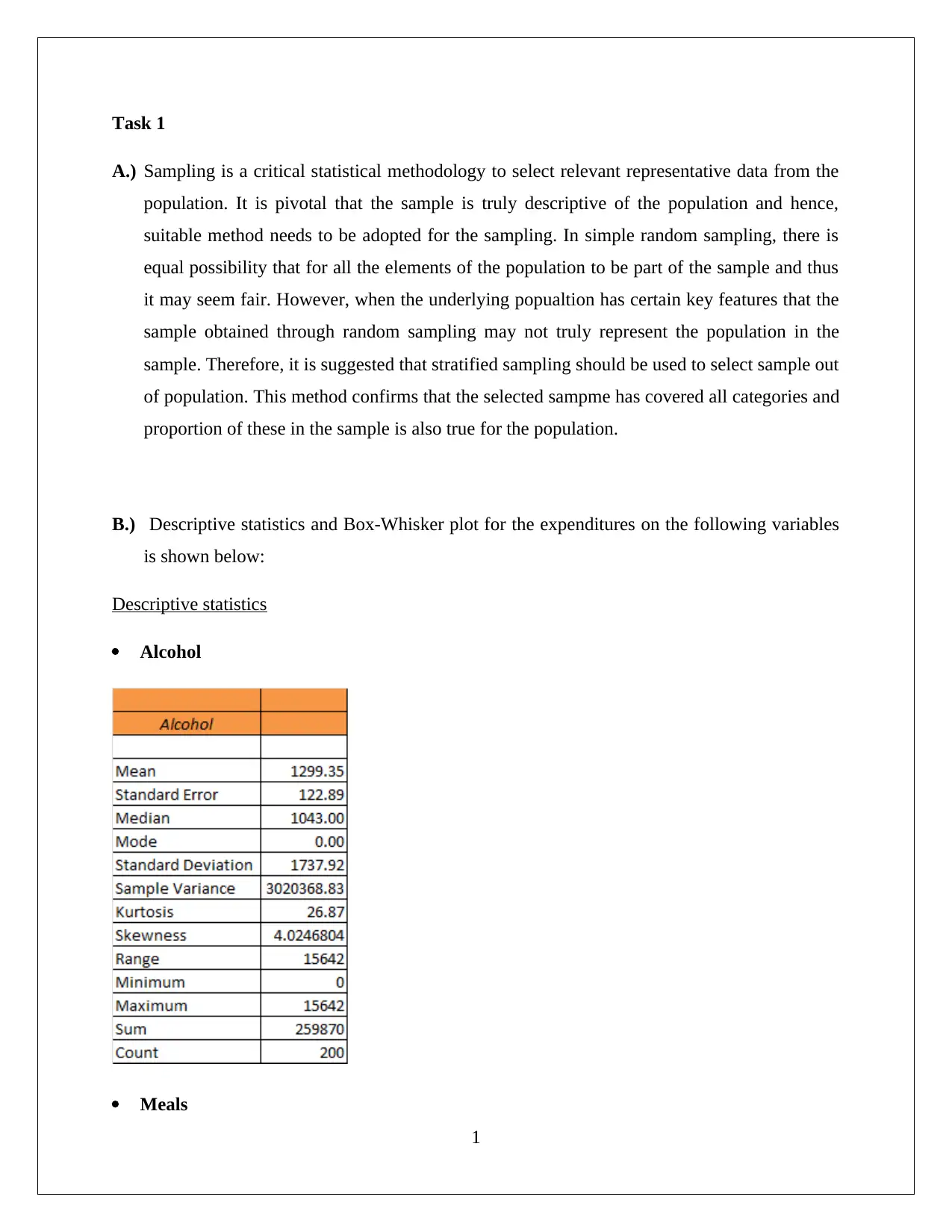
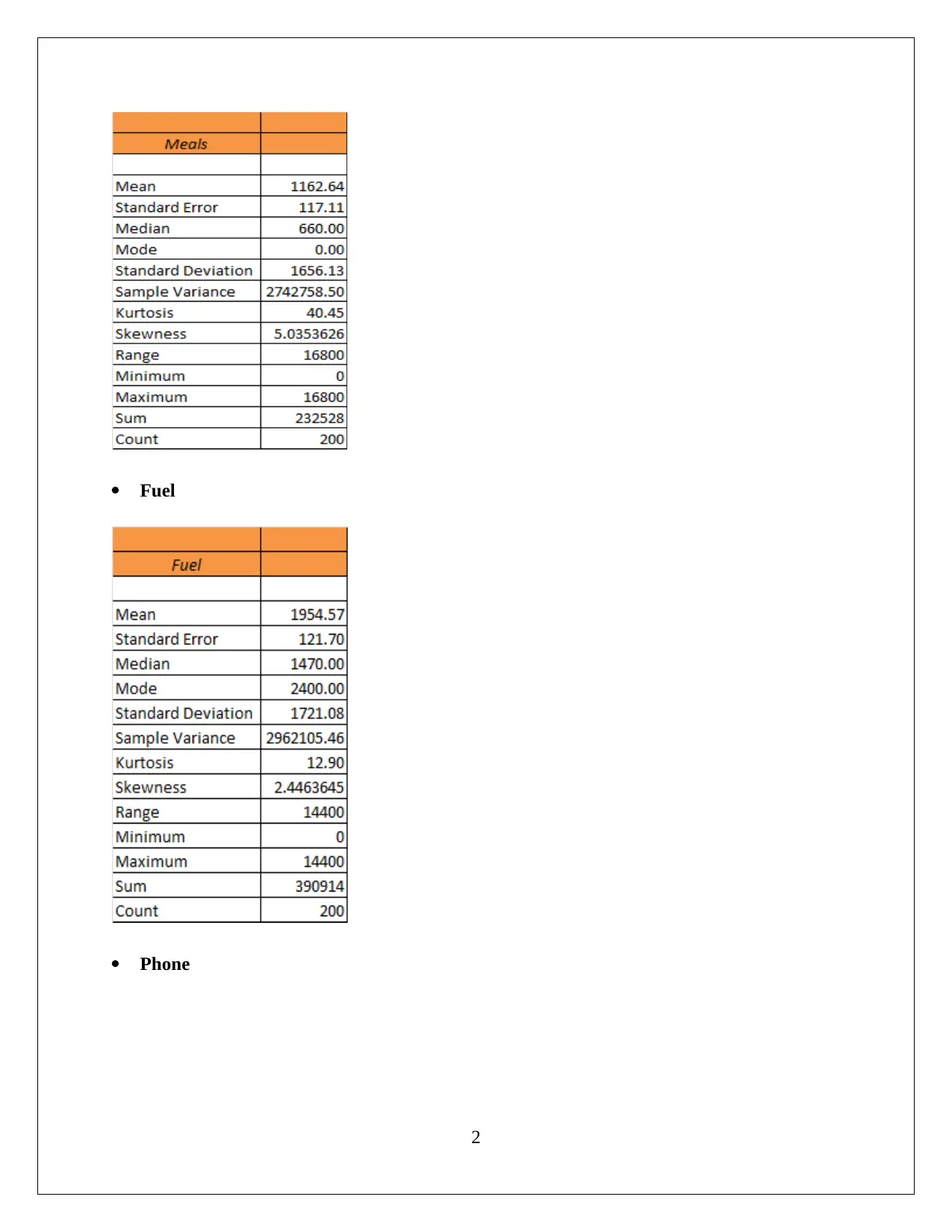
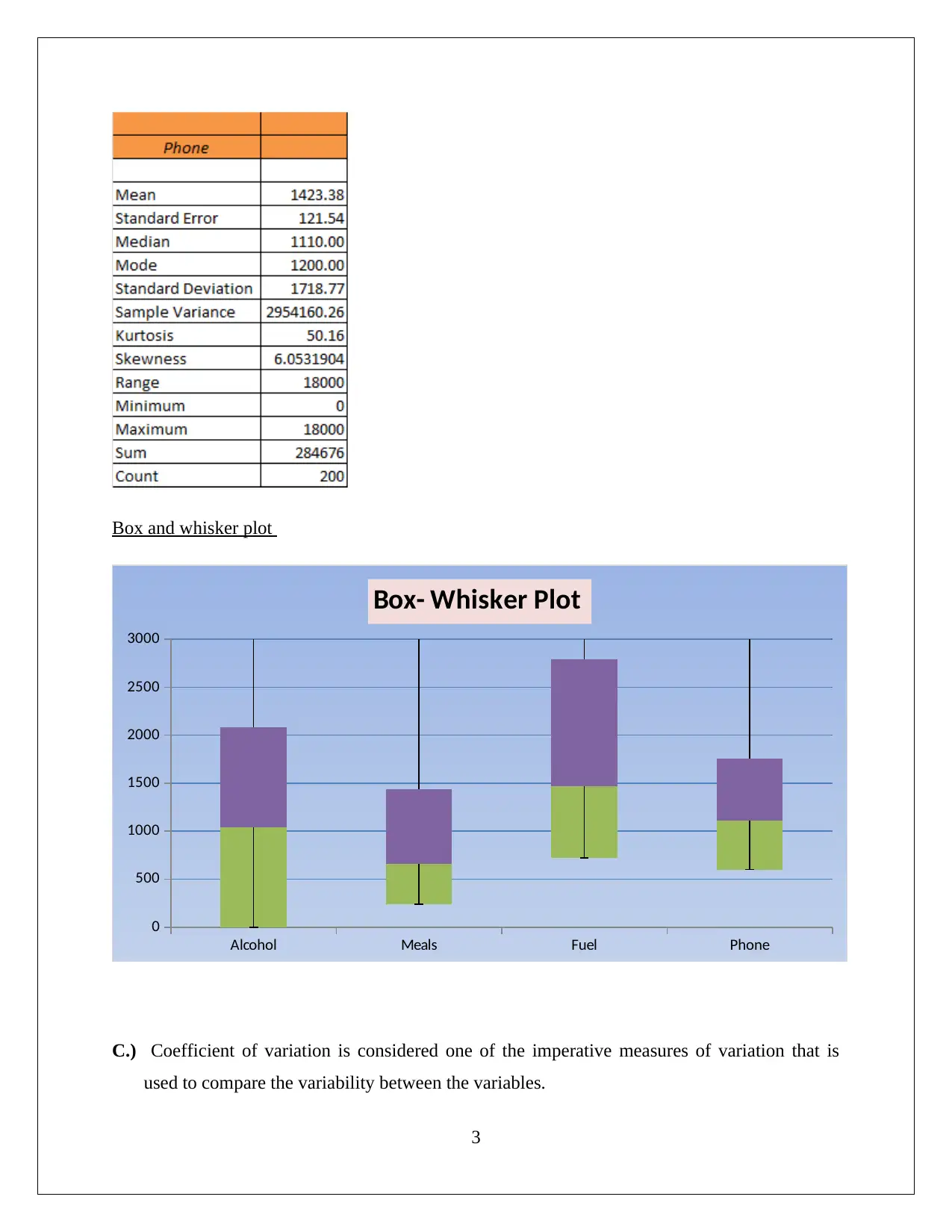
This statistics assignment analyzes household data using various statistical techniques. Task 1 focuses on sampling methods, descriptive statistics (including mean, median, mode, and skewness) for expenditures on alcohol, meals, fuel, and phone, and the use of box-whisker plots and the coefficient of variation to assess variability. Task 2 examines the frequency distribution and histogram of utility expenditures, assessing normality and skewness. Task 3 delves into household income, top and bottom income percentiles, home ownership analysis, family size probabilities, and a scatter plot and correlation analysis of income and total expenditure. Task 4 presents a contingency table analyzing the relationship between gender and education level, calculating probabilities and assessing the independence of events. The assignment demonstrates a comprehensive understanding of statistical concepts and their application to real-world data analysis, including the use of Excel for calculations and visualizations.

Statistics for Business and Finance
Assignment 1: Analysing Household Data
Student id
[Pick the date]

Task 1
A.) Sampling is a critical statistical methodology to select relevant representative data from the
population. It is pivotal that the sample is truly descriptive of the population and hence,
suitable method needs to be adopted for the sampling. In simple random sampling, there is
equal possibility that for all the elements of the population to be part of the sample and thus
it may seem fair. However, when the underlying popualtion has certain key features that the
sample obtained through random sampling may not truly represent the population in the
sample. Therefore, it is suggested that stratified sampling should be used to select sample out
of population. This method confirms that the selected sampme has covered all categories and
proportion of these in the sample is also true for the population.
B.) Descriptive statistics and Box-Whisker plot for the expenditures on the following variables
is shown below:
Descriptive statistics
 Alcohol
 Meals
1

 Fuel
 Phone
2

Box and whisker plot
Alcohol Meals Fuel Phone
0
500
1000
1500
2000
2500
3000
Box- Whisker Plot
C.) Coefficient of variation is considered one of the imperative measures of variation that is
used to compare the variability between the variables.
3

In the present case scenario, the coefficient of variation would be determined in excel with the
help of standard deviation and mean of the respective variable. Coefficient of variation (CoV) is
suitable to comment on the variability of the data because it has been determined per unit mean
of the data and hence enables comparison by eliminating the difference in mean of the variables
under consideration.
Formula used:
Coefficient of variation ¿ Standard deviation
Mean
Following conclusion can be drawn based on the above highlighted table.
 It can be said that highest variation is observed for expenditure on variable meal (CoV =
1.42).
 Lowest variation is observed for expenditure on variable fuel. (CoV = 0.88).
D. Summary
Comments on shape and spread of distribution of variables (Alcohol, meal, fuel and phone) are
highlighted below:
 Measures of central tendency: The three factors mean, median and mode of the variables are
not same. It means the distribution is not following a normal distribution.
 Presence of skew: The data would be assumed to follow a normal distribution when the value
of skew is equal to zero. All the four variables are having significantly high value of skew.
 Shape of distribution: The positive sign is the indicator of the right side tail that means the
data is having some outliers which are located at the positive side.
4

The conclusion can be drawn based on the above analysis that from the sample of 200, there are
some of the households which are spending disproportionate income on these variables.
Therefore, their expenditures on alcohol, meal, phone and fuel are high and hence, the outliers
located on the right side.
Task 2
A.) The respective frequency distribution for the “expenditure on utilities” is furnished below:
B. % of households which has spent on the utilities is computed below:
1. “%of households which have spent on the utilities at most $1200 p.a.”
¿ 25+43+ 45
200 =56.5 %
2. “% of households which have spent on the utilities between $1200 and $2400 p.a.”
¿ 30+31+12
200 =36.5 %
3. “% of households which have spent on the utilities more than $2400 p.a.”
5

¿ 8+2+4
200 =7 %
Excel output:
C. The histogram of the “expenditure occurs on the utilities by the households” is furnished
below:
Statistical reason: From the visual representation, it would be fair to conclude that the histogram
is not showing perfectly bell curve which is the representative of normal distribution. Moreover,
the long tail located on the right side of the histogram implies the non-normal distribution of
dataset and existence of “rightward skew.”
6

Task 3
A.) Variable : Household’s annual after tax income
Top and bottom 10% value of the variable has been determined by using excel inbuilt function
i.e. PERCENTILE ().
The variation between the top value and bottom value tells about the monetary position of the
extreme sections in the society. This also provides the indication of the inequality of the income
of the households.
B.) The mean of the own house is determined by using inbuilt excel function Average ().
It tells that nearly 69% of the houses are used for the residential purposes by the owners and only
31% of the houses are used for generating rent income.
C.) Family size (FS) would be the sum of total number of adults and total number of children.
The probability that the randomly taken household would have a family sizes same as five.
Total number of households = 200
Number of households that has family size exactly five = 18
7

Probability ¿ 18
200 =0.09
D.) Scatter plot in regards to comment on the association between after tax income and total
expenditure is furnished below:
Computation of coefficient of correlation has been done by taking the help of excel inbuilt
function “CORREL ().”
8

Value of correlation coefficient is higher than 0.5 but it is not near to 1 and hence, the association
between the variables is assumed to be moderate. Further, from the scatter plot, the relationship
is said to be linear because total expenditure is high at higher range of income level. However,
the non-linear behavior also present in the data which is evident from the fact that some of
households do not confer to the established pattern and tend to show a deviation in their
behavior.
Task 4
A.) “Contingency table - gender and level of education”
It can be said from the table that distribution of highest degree between male and female head of
household are different. This is also evident from the Chi-square test.
B.) “Probability (Female head of household, Intermediate highest degree)” ¿ 9
200 =0.045
C.) “Probability (Male head of household, Bachelor highest degree) ¿ 13
200 =0.065
D.) “Proportion (Secondary highest degree among females)” = 22
102=0.215
E.) Events “Gender of the household is male” and “having the Masters Degree” would be
assumed only if
9

P ( G )=“ ‘ Gender of the household is male ’= 98
200 =0.49
P ( H )=“ having the Masters Degree”=37/200=0.185
P ( G∧H )= 23
200 =0.115
G and H would be independent if
P ( G∧H ) =P ( G ) ∗P ( H )
0.115= ( 0.49 )∗ ( 0.185 )
0.115 ≠ 0.090
Hence, “the events are not independent”
10