Statistics Homework: Data Analysis, Probability, Misconceptions

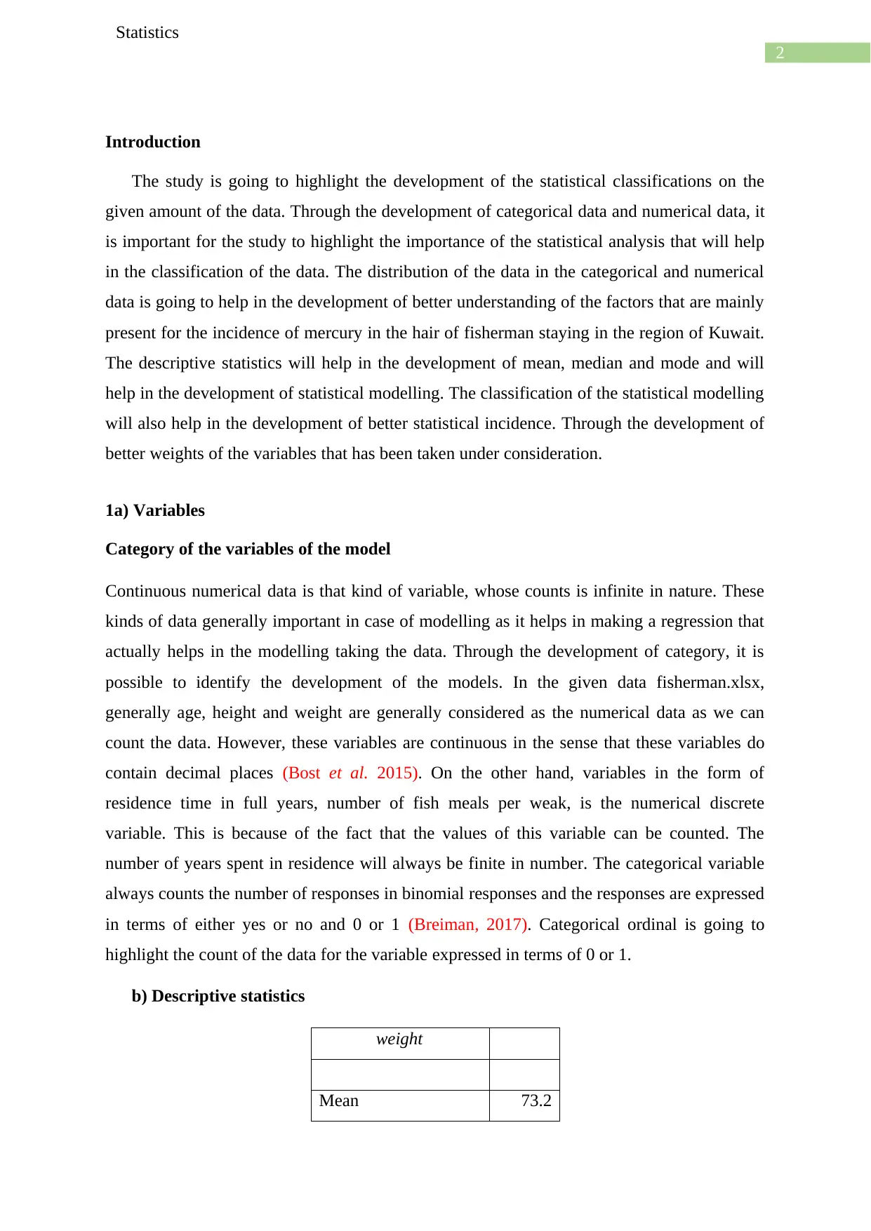
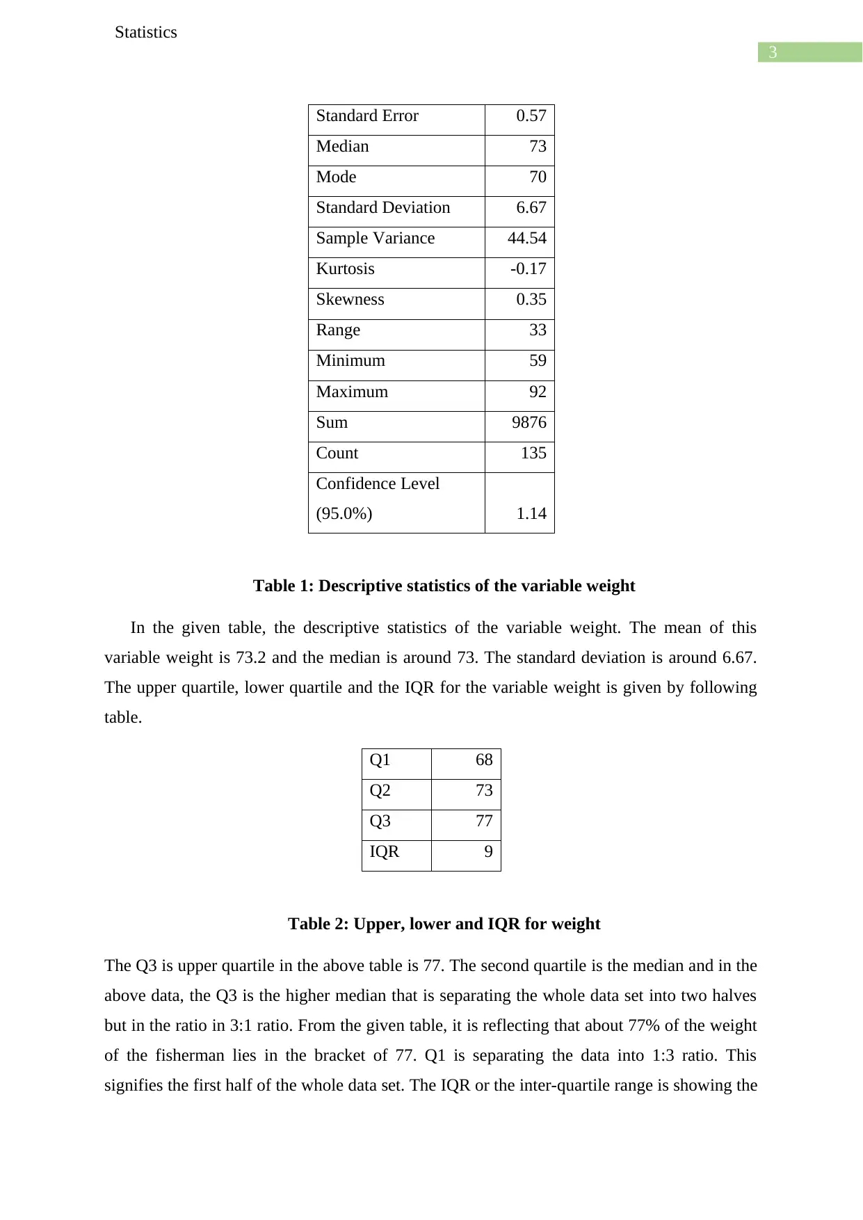
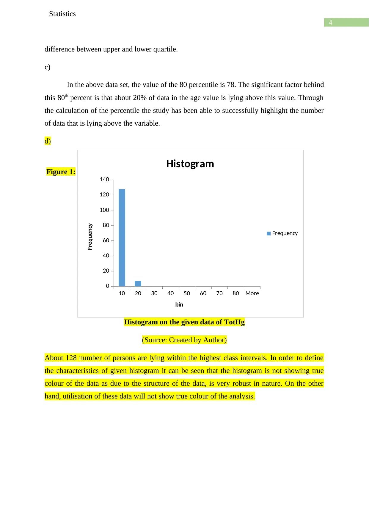
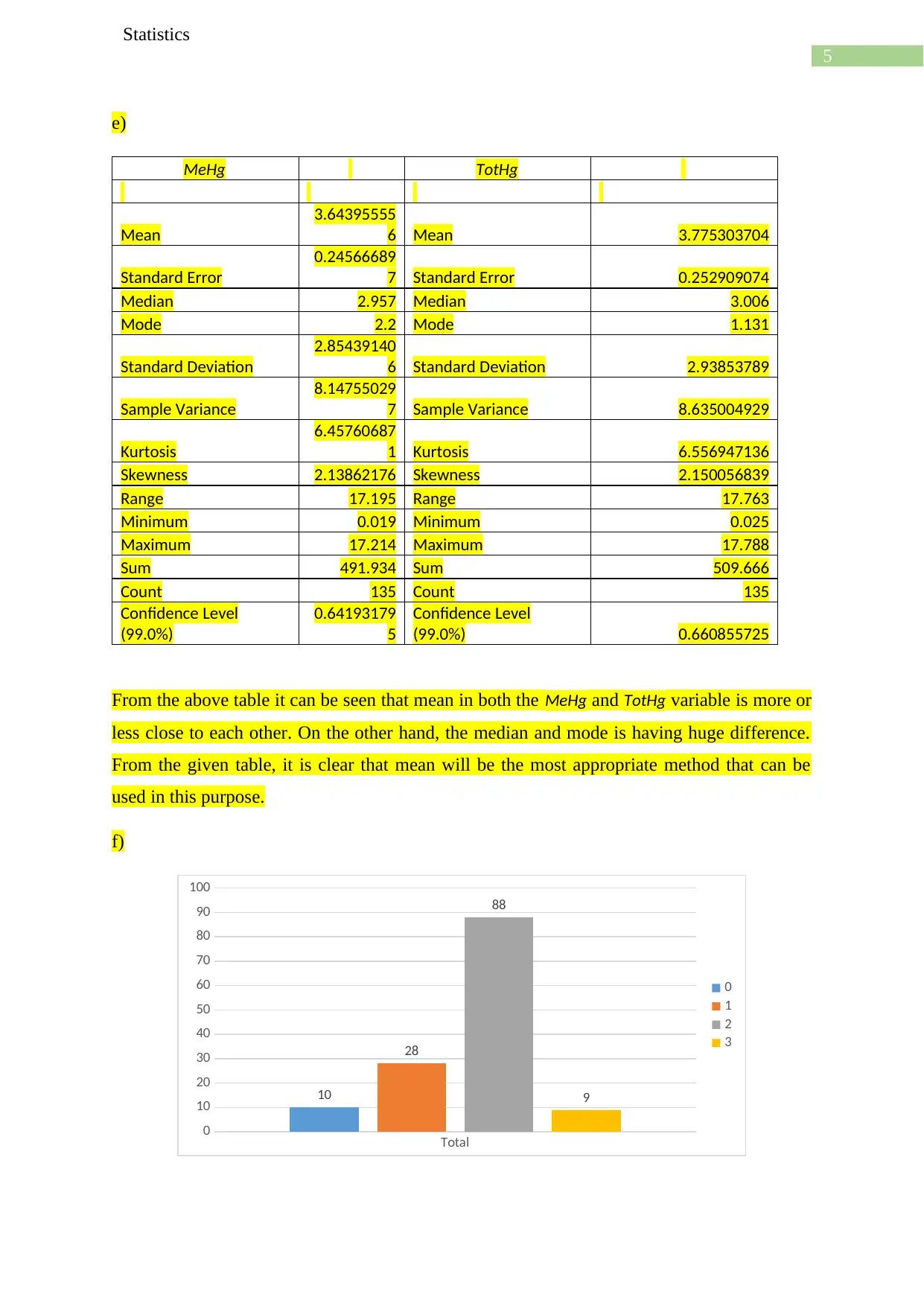
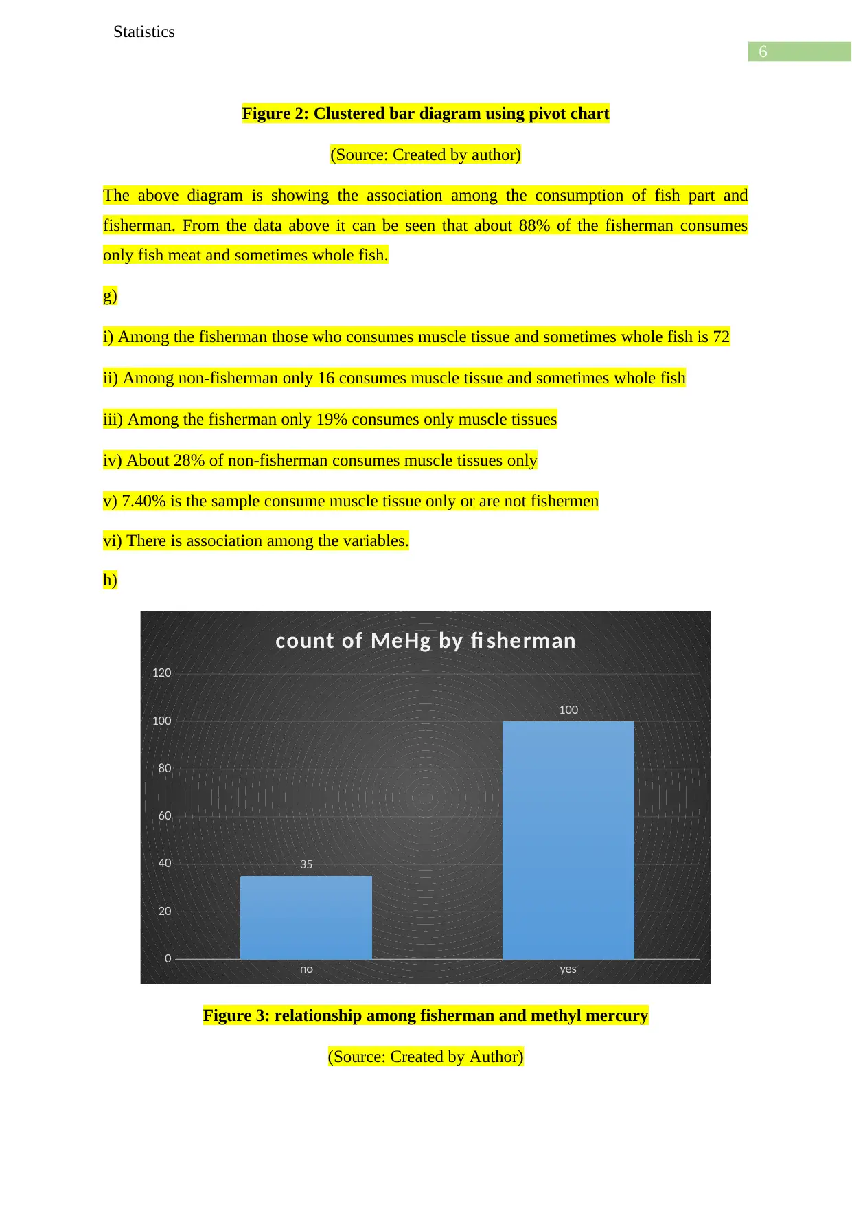
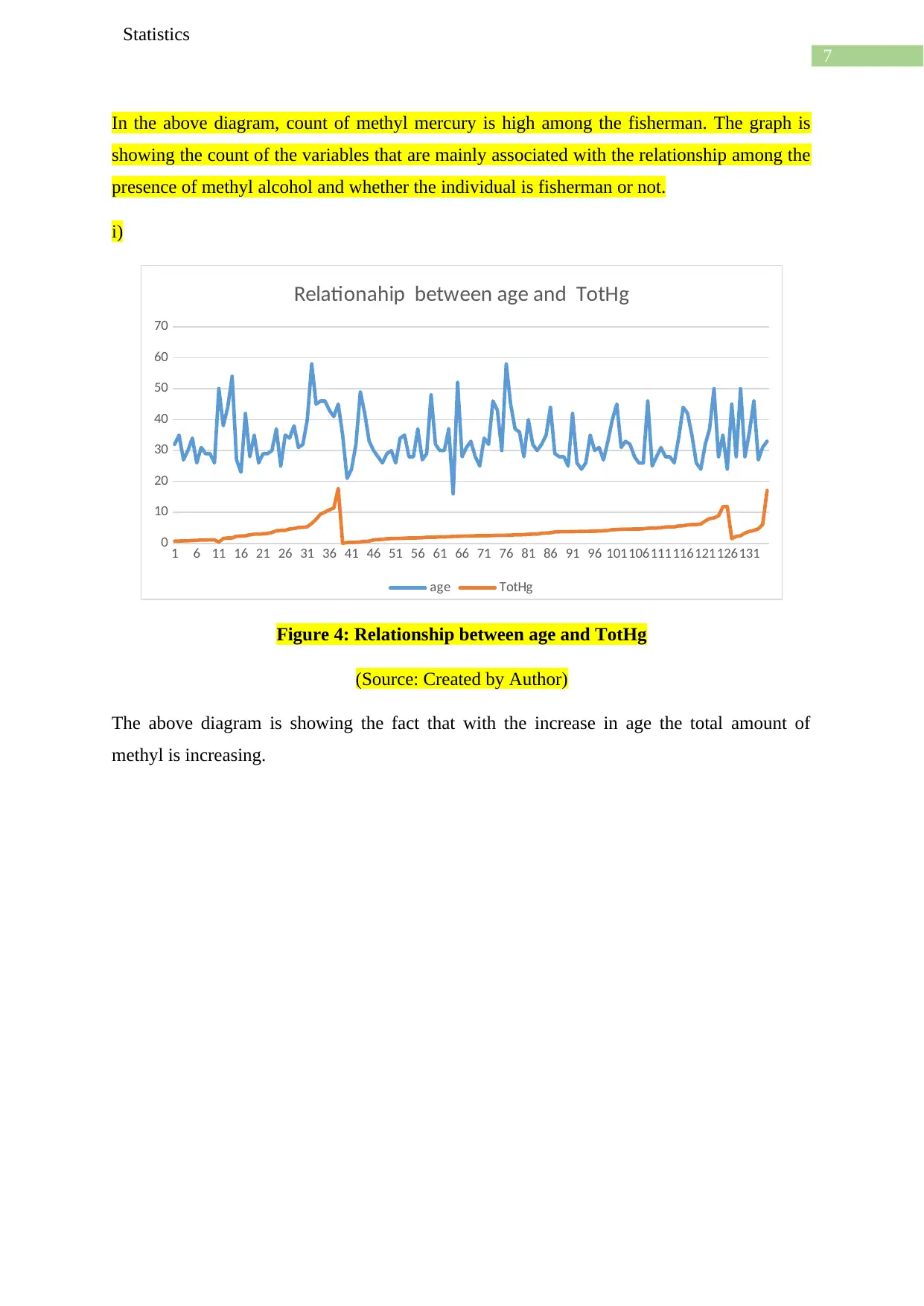
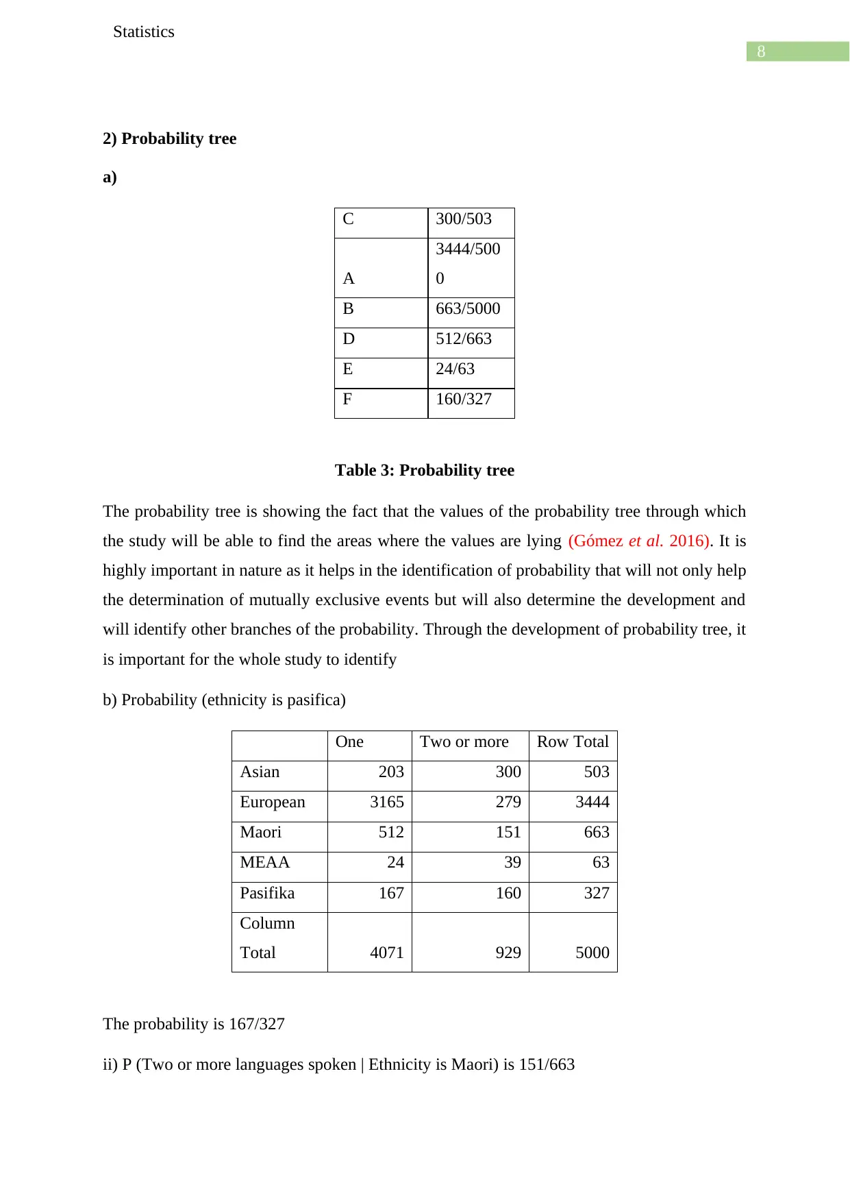
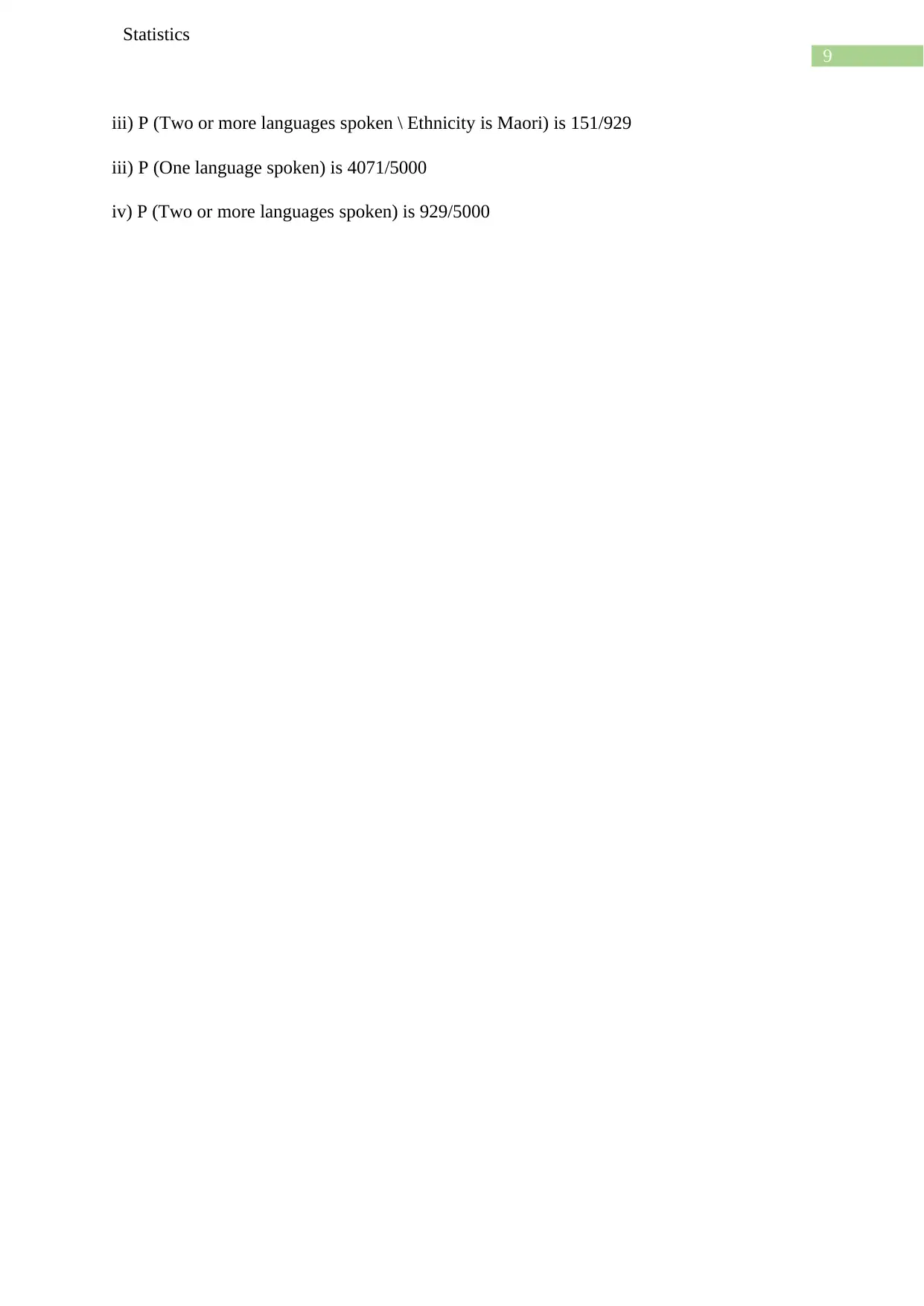
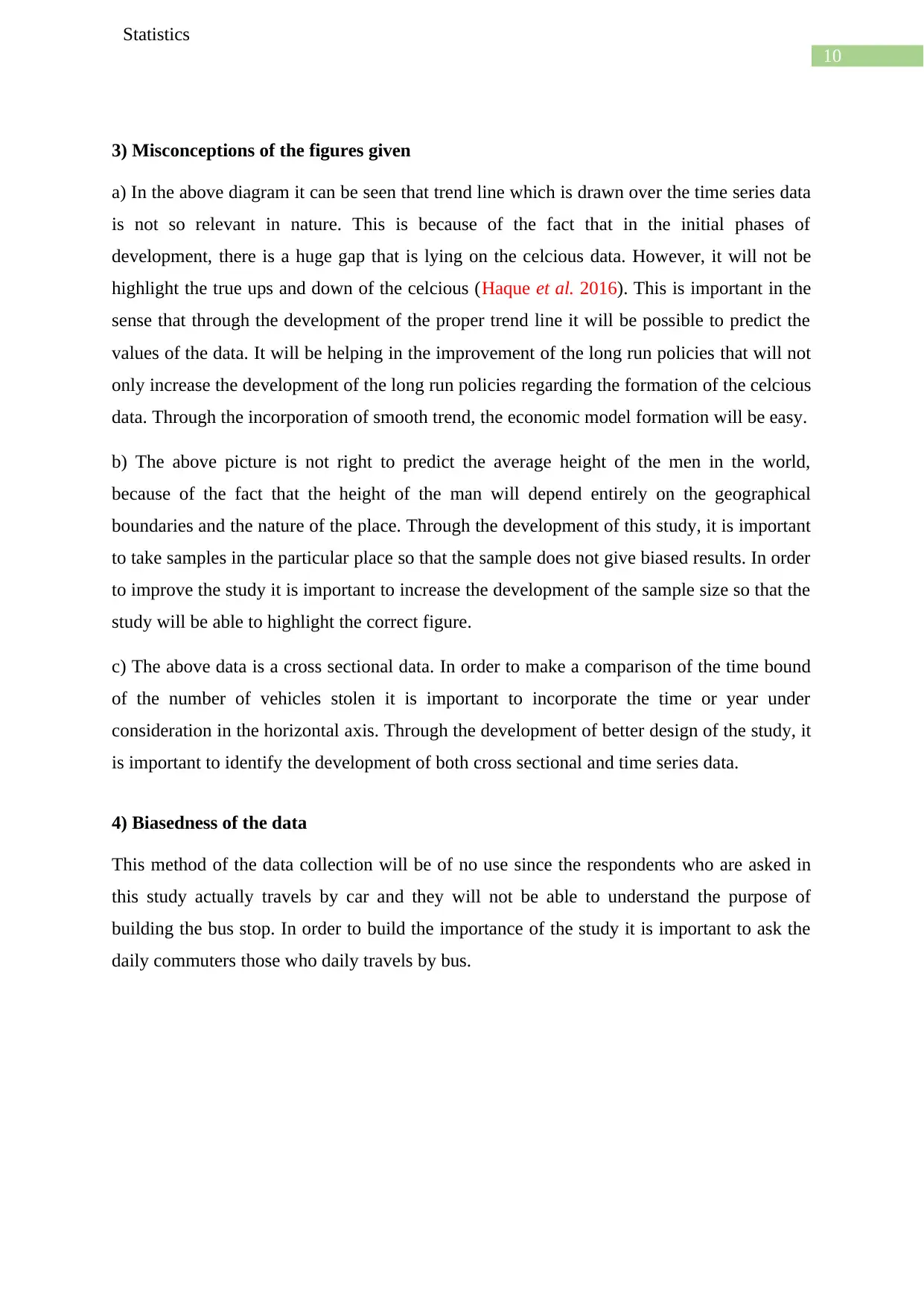
This statistics assignment provides a detailed analysis of a dataset related to mercury levels in fishermen. It covers various aspects of statistical analysis, including the classification of variables into continuous numerical, discrete numerical, and categorical types. Descriptive statistics such as mean, median, standard deviation, and quartiles are calculated for the 'weight' variable. The assignment also includes the creation and interpretation of a histogram for 'TotHg' data, along with a comparative analysis of 'MeHg' and 'TotHg' variables. Furthermore, it explores the association between fish consumption habits and fishermen status using clustered bar diagrams and pivot charts. The assignment delves into probability calculations using a probability tree and addresses common misconceptions in statistical figures. The solution is available on Desklib, where students can find additional resources like past papers and solved assignments.

Running head: Statistics
Statistics
Name of the course
Name of Student
Course ID:

1
Statistics
Table of Contents
Introduction................................................................................................................................2
1a) Variables..............................................................................................................................2
2) Probability tree.......................................................................................................................5
3) Misconceptions of the figures given......................................................................................6
4) Biasedness of the data............................................................................................................6

2
Statistics
Introduction
The study is going to highlight the development of the statistical classifications on the
given amount of the data. Through the development of categorical data and numerical data, it
is important for the study to highlight the importance of the statistical analysis that will help
in the classification of the data. The distribution of the data in the categorical and numerical
data is going to help in the development of better understanding of the factors that are mainly
present for the incidence of mercury in the hair of fisherman staying in the region of Kuwait.
The descriptive statistics will help in the development of mean, median and mode and will
help in the development of statistical modelling. The classification of the statistical modelling
will also help in the development of better statistical incidence. Through the development of
better weights of the variables that has been taken under consideration.
1a) Variables
Category of the variables of the model
Continuous numerical data is that kind of variable, whose counts is infinite in nature. These
kinds of data generally important in case of modelling as it helps in making a regression that
actually helps in the modelling taking the data. Through the development of category, it is
possible to identify the development of the models. In the given data fisherman.xlsx,
generally age, height and weight are generally considered as the numerical data as we can
count the data. However, these variables are continuous in the sense that these variables do
contain decimal places (Bost et al. 2015). On the other hand, variables in the form of
residence time in full years, number of fish meals per weak, is the numerical discrete
variable. This is because of the fact that the values of this variable can be counted. The
number of years spent in residence will always be finite in number. The categorical variable
always counts the number of responses in binomial responses and the responses are expressed
in terms of either yes or no and 0 or 1 (Breiman, 2017). Categorical ordinal is going to
highlight the count of the data for the variable expressed in terms of 0 or 1.
b) Descriptive statistics
weight
Mean 73.2

3
Statistics
Standard Error 0.57
Median 73
Mode 70
Standard Deviation 6.67
Sample Variance 44.54
Kurtosis -0.17
Skewness 0.35
Range 33
Minimum 59
Maximum 92
Sum 9876
Count 135
Confidence Level
(95.0%) 1.14
Table 1: Descriptive statistics of the variable weight
In the given table, the descriptive statistics of the variable weight. The mean of this
variable weight is 73.2 and the median is around 73. The standard deviation is around 6.67.
The upper quartile, lower quartile and the IQR for the variable weight is given by following
table.
Q1 68
Q2 73
Q3 77
IQR 9
Table 2: Upper, lower and IQR for weight
The Q3 is upper quartile in the above table is 77. The second quartile is the median and in the
above data, the Q3 is the higher median that is separating the whole data set into two halves
but in the ratio in 3:1 ratio. From the given table, it is reflecting that about 77% of the weight
of the fisherman lies in the bracket of 77. Q1 is separating the data into 1:3 ratio. This
signifies the first half of the whole data set. The IQR or the inter-quartile range is showing the

4
Statistics
difference between upper and lower quartile.
c)
In the above data set, the value of the 80 percentile is 78. The significant factor behind
this 80th percent is that about 20% of data in the age value is lying above this value. Through
the calculation of the percentile the study has been able to successfully highlight the number
of data that is lying above the variable.
d)
Figure 1:
Histogram on the given data of TotHg
(Source: Created by Author)
About 128 number of persons are lying within the highest class intervals. In order to define
the characteristics of given histogram it can be seen that the histogram is not showing true
colour of the data as due to the structure of the data, is very robust in nature. On the other
hand, utilisation of these data will not show true colour of the analysis.
10 20 30 40 50 60 70 80 More
0
20
40
60
80
100
120
140
Histogram
Frequency
bin
Frequency

5
Statistics
e)
MeHg TotHg
Mean
3.64395555
6 Mean 3.775303704
Standard Error
0.24566689
7 Standard Error 0.252909074
Median 2.957 Median 3.006
Mode 2.2 Mode 1.131
Standard Deviation
2.85439140
6 Standard Deviation 2.93853789
Sample Variance
8.14755029
7 Sample Variance 8.635004929
Kurtosis
6.45760687
1 Kurtosis 6.556947136
Skewness 2.13862176 Skewness 2.150056839
Range 17.195 Range 17.763
Minimum 0.019 Minimum 0.025
Maximum 17.214 Maximum 17.788
Sum 491.934 Sum 509.666
Count 135 Count 135
Confidence Level
(99.0%)
0.64193179
5
Confidence Level
(99.0%) 0.660855725
From the above table it can be seen that mean in both the MeHg and TotHg variable is more or
less close to each other. On the other hand, the median and mode is having huge difference.
From the given table, it is clear that mean will be the most appropriate method that can be
used in this purpose.
f)
Total
0
10
20
30
40
50
60
70
80
90
100
10
28
88
9
0
1
2
3

6
Statistics
Figure 2: Clustered bar diagram using pivot chart
(Source: Created by author)
The above diagram is showing the association among the consumption of fish part and
fisherman. From the data above it can be seen that about 88% of the fisherman consumes
only fish meat and sometimes whole fish.
g)
i) Among the fisherman those who consumes muscle tissue and sometimes whole fish is 72
ii) Among non-fisherman only 16 consumes muscle tissue and sometimes whole fish
iii) Among the fisherman only 19% consumes only muscle tissues
iv) About 28% of non-fisherman consumes muscle tissues only
v) 7.40% is the sample consume muscle tissue only or are not fishermen
vi) There is association among the variables.
h)
no yes
0
20
40
60
80
100
120
35
100
count of MeHg by fi sherman
Figure 3: relationship among fisherman and methyl mercury
(Source: Created by Author)

7
Statistics
In the above diagram, count of methyl mercury is high among the fisherman. The graph is
showing the count of the variables that are mainly associated with the relationship among the
presence of methyl alcohol and whether the individual is fisherman or not.
i)
1 6 11 16 21 26 31 36 41 46 51 56 61 66 71 76 81 86 91 96 101106111116121126131
0
10
20
30
40
50
60
70
Relationahip between age and TotHg
age TotHg
Figure 4: Relationship between age and TotHg
(Source: Created by Author)
The above diagram is showing the fact that with the increase in age the total amount of
methyl is increasing.

8
Statistics
2) Probability tree
a)
C 300/503
A
3444/500
0
B 663/5000
D 512/663
E 24/63
F 160/327
Table 3: Probability tree
The probability tree is showing the fact that the values of the probability tree through which
the study will be able to find the areas where the values are lying (Gómez et al. 2016). It is
highly important in nature as it helps in the identification of probability that will not only help
the determination of mutually exclusive events but will also determine the development and
will identify other branches of the probability. Through the development of probability tree, it
is important for the whole study to identify
b) Probability (ethnicity is pasifica)
One Two or more Row Total
Asian 203 300 503
European 3165 279 3444
Maori 512 151 663
MEAA 24 39 63
Pasifika 167 160 327
Column
Total 4071 929 5000
The probability is 167/327
ii) P (Two or more languages spoken | Ethnicity is Maori) is 151/663

9
Statistics
iii) P (Two or more languages spoken \ Ethnicity is Maori) is 151/929
iii) P (One language spoken) is 4071/5000
iv) P (Two or more languages spoken) is 929/5000

10
Statistics
3) Misconceptions of the figures given
a) In the above diagram it can be seen that trend line which is drawn over the time series data
is not so relevant in nature. This is because of the fact that in the initial phases of
development, there is a huge gap that is lying on the celcious data. However, it will not be
highlight the true ups and down of the celcious (Haque et al. 2016). This is important in the
sense that through the development of the proper trend line it will be possible to predict the
values of the data. It will be helping in the improvement of the long run policies that will not
only increase the development of the long run policies regarding the formation of the celcious
data. Through the incorporation of smooth trend, the economic model formation will be easy.
b) The above picture is not right to predict the average height of the men in the world,
because of the fact that the height of the man will depend entirely on the geographical
boundaries and the nature of the place. Through the development of this study, it is important
to take samples in the particular place so that the sample does not give biased results. In order
to improve the study it is important to increase the development of the sample size so that the
study will be able to highlight the correct figure.
c) The above data is a cross sectional data. In order to make a comparison of the time bound
of the number of vehicles stolen it is important to incorporate the time or year under
consideration in the horizontal axis. Through the development of better design of the study, it
is important to identify the development of both cross sectional and time series data.
4) Biasedness of the data
This method of the data collection will be of no use since the respondents who are asked in
this study actually travels by car and they will not be able to understand the purpose of
building the bus stop. In order to build the importance of the study it is important to ask the
daily commuters those who daily travels by bus.

11
Statistics
Reference list
Bost, R., Popa, R.A., Tu, S. and Goldwasser, S., 2015, February. Machine learning
classification over encrypted data. In NDSS (Vol. 4324, p. 4325).
Breiman, L., 2017. Classification and regression trees. Routledge.
Gómez, C., White, J.C. and Wulder, M.A., 2016. Optical remotely sensed time series data for
land cover classification: A review. ISPRS Journal of Photogrammetry and Remote
Sensing, 116, pp.55-72.
Haque, A., Khan, L. and Baron, M., 2016, February. Sand: Semi-supervised adaptive novel
class detection and classification over data stream. In THIRTIETH AAAI Conference on
Artificial Intelligence.
Qi, C.R., Su, H., Nießner, M., Dai, A., Yan, M. and Guibas, L.J., 2016. Volumetric and
multi-view cnns for object classification on 3d data. In Proceedings of the IEEE conference
on computer vision and pattern recognition (pp. 5648-5656).
Salamon, J. and Bello, J.P., 2017. Deep convolutional neural networks and data augmentation
for environmental sound classification. IEEE Signal Processing Letters, 24(3), pp.279-283.
Tennant, M., Stahl, F., Rana, O. and Gomes, J.B., 2017. Scalable real-time classification of
data streams with concept drift. Future Generation Computer Systems, 75, pp.187-199.
Wong, S.C., Gatt, A., Stamatescu, V. and McDonnell, M.D., 2016, November. Understanding
data augmentation for classification: when to warp?. In 2016 international conference on
digital image computing: techniques and applications (DICTA) (pp. 1-6). IEEE.