Statistics Assignment: Data Analysis, Probability and Solutions
VerifiedAdded on 2023/04/23
|11
|1066
|354
Homework Assignment
AI Summary
This statistics assignment covers a range of topics including descriptive statistics, probability, and hypothesis testing. It includes stem and leaf plots, frequency polygons, bar charts, and comparisons of stock data. The assignment also involves calculating mean, standard deviation, quartiles, and creating box-whisker plots. Probability calculations are performed for various scenarios, including household internet access and bus arrival times. Hypothesis testing is conducted to analyze flight booking cancellations. Confidence intervals are calculated. Numerical solutions and interpretations are provided for each question. Find more solved assignments and study resources on Desklib.

STUDENT ID:
Paraphrase This Document
Need a fresh take? Get an instant paraphrase of this document with our AI Paraphraser

Question 1
Part a) Quarterly opening prices for NAB (National Australia Bank) and WBC (Westpac
Banking Corporation)
Stem and leaf plot
Part b) Frequency polygon and relative frequency histogram
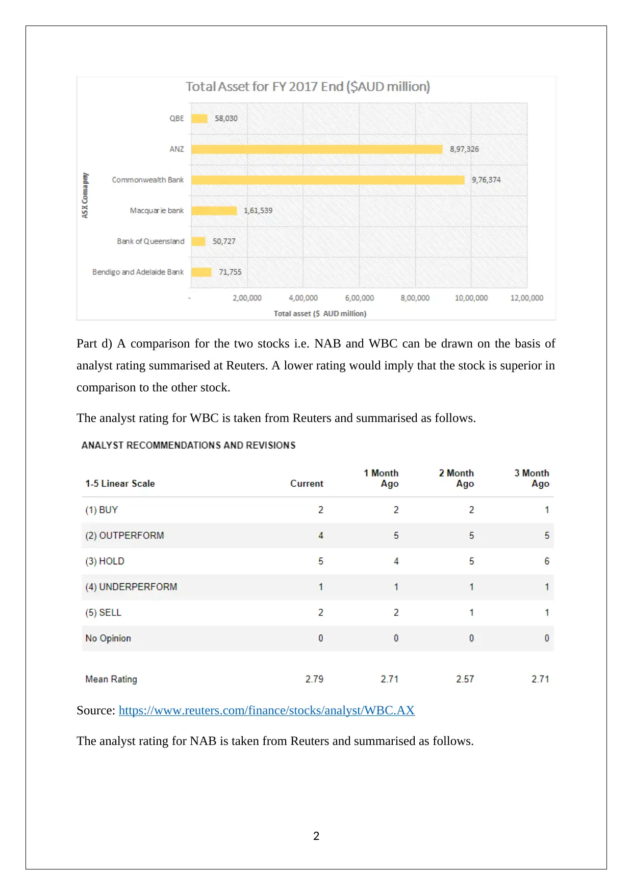
Part c) Bar chart for total assets of the six ASX listed companies.
1
Part a) Quarterly opening prices for NAB (National Australia Bank) and WBC (Westpac
Banking Corporation)
Stem and leaf plot
Part b) Frequency polygon and relative frequency histogram
Part c) Bar chart for total assets of the six ASX listed companies.
1

Part d) A comparison for the two stocks i.e. NAB and WBC can be drawn on the basis of
analyst rating summarised at Reuters. A lower rating would imply that the stock is superior in
comparison to the other stock.
The analyst rating for WBC is taken from Reuters and summarised as follows.
Source: https://www.reuters.com/finance/stocks/analyst/WBC.AX
The analyst rating for NAB is taken from Reuters and summarised as follows.
2
⊘ This is a preview!⊘
Do you want full access?
Subscribe today to unlock all pages.

Trusted by 1+ million students worldwide

Source: https://www.reuters.com/finance/stocks/analyst/NAB.AX
Comparing the two mean ratings in the present, it is apparent that a lower rating is indicated for
NAB when compared to WBC. This clearly implies that the superior stock worth buying is NAB.
Question 2
Part a) Mean and standard deviation is computed through excel functions as shown below.
Mean = AVERAGE ()
Standard deviation = STDEV ()
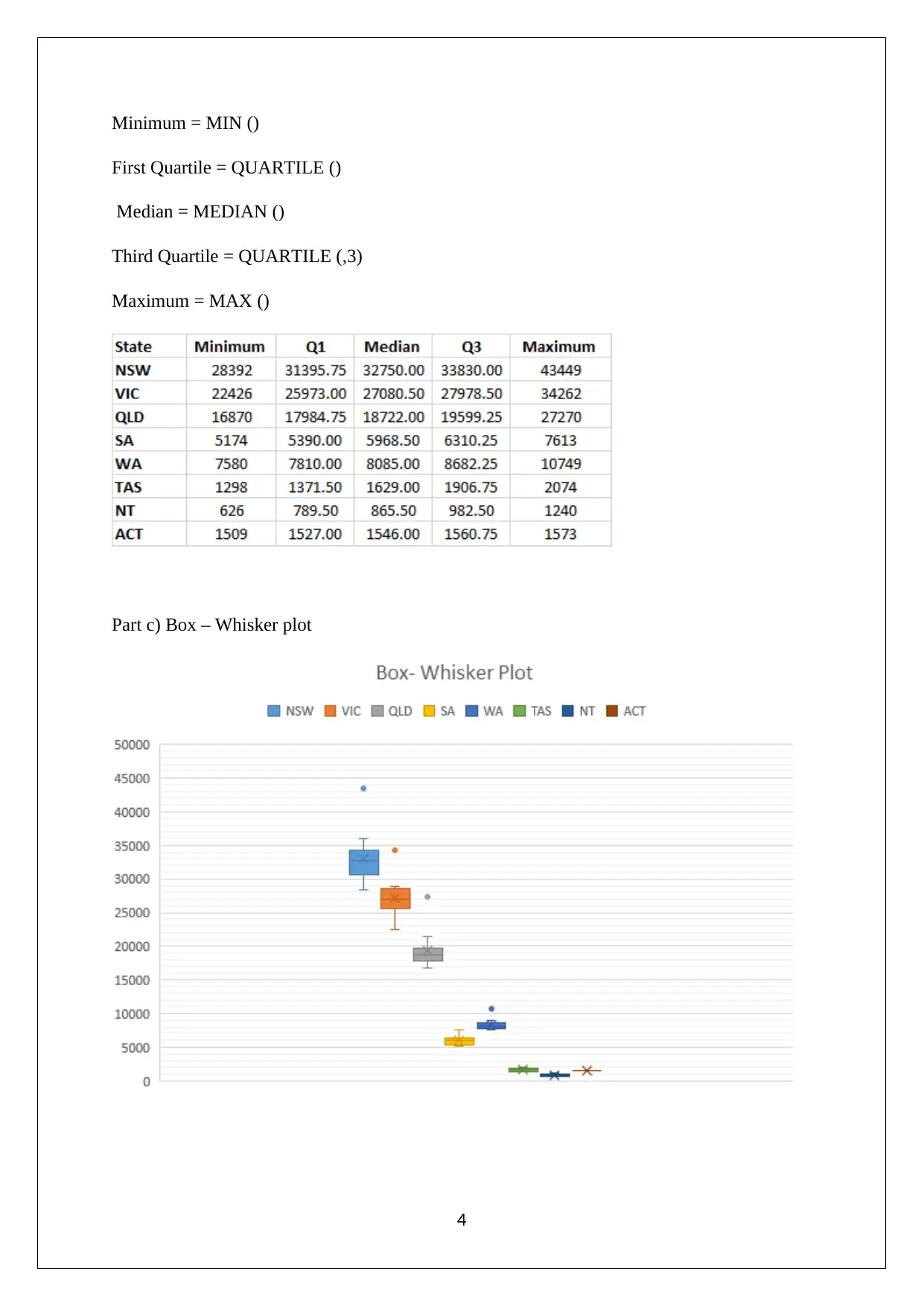
Part b) Minimum, maximum Q1, Q3 and medianis computed through excel functions as
shown below.
3
Paraphrase This Document
Need a fresh take? Get an instant paraphrase of this document with our AI Paraphraser

Minimum = MIN ()
First Quartile = QUARTILE ()
Median = MEDIAN ()
Third Quartile = QUARTILE (,3)
Maximum = MAX ()
Part c) Box – Whisker plot
4
First Quartile = QUARTILE ()
Median = MEDIAN ()
Third Quartile = QUARTILE (,3)
Maximum = MAX ()
Part c) Box – Whisker plot
4

Part d) The new vehicles sale shows a significant amount of variation across the given states.
However, NSW & Victoria are the two leading states with regards to new vehicles sales. This
does not come as a surprise since the above states house higher population and also have
Sydney and Melbourne. Another crucial observation is that for every state, the highest new
vehicle sale is observed in June.
Question 3
Row and column totals have been computed.
Part a) Probability (household: Victoria) =8925.10/35466.1=0.252
Part b) Probability (household: Tasmania, Internet access, 2010-2011) =146.2/6723.6=0.022
Partc) Probability (household: New South wales, Internet access, 2012-
2013)=2274.5/35466.1=0.064
Part d) Probability (household:Internet access, 2010-2011 or 2012-
2013)=(6723.6+7343.2)/35466.1=0.397
Question 4
Part a) Average arrival time for the bus μ=73 min
Standard deviation of the arrival time for the bus σ =8 min
Assume that the upper 5% of the total time exceeds = x
5
⊘ This is a preview!⊘
Do you want full access?
Subscribe today to unlock all pages.

Trusted by 1+ million students worldwide

When 5% of the total time exceeds x then the corresponding cumulative probability would
become 0.95. Therefore, the z value corresponding to 0.95 probability would be 1.6448
(Hillier, 2016).
Now,
The formula for z value
z= x−μ
σ =1.644 8= x −73
8
x=86.16 minutes
Part b) It is apparent that the deviation of the temperature between the two temperature T1
=120 C and T2=250C is uniform. Therefore, it can be said that 100% of temperature values
would be existed within 130C of the T1. Hence, 210C would be 90C higher than T1.
Now,
130C has 100% values, 10C has (100/13) % of the values and 70C has ((100*7)/13)%
Therefore, the probability that the temperature will be lesser than 21 0C= ((100*7)/13) %
=0.5385
Part c) (i) Expected probability of distinguish = 0.50
Standard deviation ¿ √ ( 0.5∗(1−0.5)
200 )=0.0353
z= x−μ
σ = 0.65−0.50
0.0353 =4.249
From standard normal table,
P ( z ≤ 4.249 ) =0.00001
There is a 0.0001 probability that more than 65% of the total respondents would able to
distinguish.
6
Paraphrase This Document
Need a fresh take? Get an instant paraphrase of this document with our AI Paraphraser

(ii) Probability that the sample will have between 50% and 60% of identifications correct.
P ( 50 %< x <60 % )=P ( 0.5−0.50
0.0353 < z< 0.6−0.50
0.0353 )=P ( 0< z< 2.832 )
From standard normal table,
P ( z< 2.832 )=0.9976
P ( z< 0 )=0.5
Hence,
P ( 50 %<x <60 % ) =0.9976−0.5=0.498
Question 5
Part a) There are 500 trials and 0.70 probability for success.
Normal approximation of binomial distribution
μ=0.70∗500=350
σ = √ ( 500∗0.3∗0.7 )=10.25
Now,
P ( 280< x< 355 ) =0.688
Part b) Number of travellers are 500 and there are 210 travellers who have later cancel their
flights booking.
Hypothesis testing
H0 : p >¿ 0.50
Ha : p <0.50
Requisite proportion ¿ 210
500 =0.42
7

Standard error = sqrt (p* (1-p) /n) = sqrt (0.50*0.5/500) = 0.02236
Z value ¿ 0.42−0.50
0.02236 =−3.57
The p value = 0.0002
The alpha (significance level) = 1%
It is evident that p value is lower than alpha and hence, null hypothesis will be rejected and
alternative hypothesis will be adopted (Fehr & Grossman, 2014). Thus. It can be concluded
that proportion of travellers who have later cancel their flights booking is lower than 50% is
true.
Part c) 95% confidence interval
μ= 911
9 =101.2
Standard deviation= √ ( 3831.556
9−1 )=21.8
Standard error = 21.8/ sqrt (9) = 7.29
8
⊘ This is a preview!⊘
Do you want full access?
Subscribe today to unlock all pages.

Trusted by 1+ million students worldwide

Degree of freedom (dof) = 9 -1 = 8
The t value = 2.31
Margin of error = 2.31 * 7.29 =16.839
Lower limit = Mean – Margin of error = 101.2 – 16.839 = 84.36
Upper limit = Mean + Margin of error = 101.2 + 16.839 = 118.03
9
The t value = 2.31
Margin of error = 2.31 * 7.29 =16.839
Lower limit = Mean – Margin of error = 101.2 – 16.839 = 84.36
Upper limit = Mean + Margin of error = 101.2 + 16.839 = 118.03
9
Paraphrase This Document
Need a fresh take? Get an instant paraphrase of this document with our AI Paraphraser

References
Fehr, F. H., & Grossman, G. (2014). An introduction to sets, probability and hypothesis
testing (3rd ed.). Ohio: Heath.
Hillier, F. (2016). Introduction to Operations Research. (6th ed.). New York: McGraw Hill
Publications.
10
Fehr, F. H., & Grossman, G. (2014). An introduction to sets, probability and hypothesis
testing (3rd ed.). Ohio: Heath.
Hillier, F. (2016). Introduction to Operations Research. (6th ed.). New York: McGraw Hill
Publications.
10
1 out of 11
Your All-in-One AI-Powered Toolkit for Academic Success.
+13062052269
info@desklib.com
Available 24*7 on WhatsApp / Email
![[object Object]](/_next/static/media/star-bottom.7253800d.svg)
Unlock your academic potential
Copyright © 2020–2026 A2Z Services. All Rights Reserved. Developed and managed by ZUCOL.

