Statistics Report: Data Analysis and Interpretation - Statistics
VerifiedAdded on 2020/07/22
|19
|3281
|322
Report
AI Summary
This report presents a comprehensive statistical analysis of data from both public and private sectors, focusing on earnings, pay gaps, and various business metrics. It begins with an identification of changes in gross annual earnings and gender pay gaps, followed by an analysis using ogive charts to determine mean and standard deviation. The report further explores the relationship between size and turnover in retail settings through scatter diagrams, correlation coefficients, and regression analysis, including predictions and statistical validity assessments. Additionally, it addresses economic order quantity and its cost implications. The analysis includes multiple tables and figures to support the interpretations and conclusions drawn, offering valuable insights into the trends and relationships within the data.
STATISTICS MANAGEMENT
Paraphrase This Document
Need a fresh take? Get an instant paraphrase of this document with our AI Paraphraser
TABLE OF CONTENTS
INTRODUCTION...........................................................................................................................1
TASK 1............................................................................................................................................1
(a)Identifcation of change in gross annual earnings in public and private sector since 2009 and
pay gap across genders................................................................................................................1
TASK 2............................................................................................................................................4
(a)Ogive chart and computation of mean as well as standard deviation.....................................4
(b) Comparison of earning of two regions...................................................................................6
(a)Area and average weekly turnover scatter diagram and reltionship between them................7
© Equation used for making prediction.....................................................................................10
(e) Statistical validity of model..................................................................................................10
TASK 3..........................................................................................................................................11
(a)Number of delieveries made each year by firm....................................................................11
(b) Number of bootles of olive oil sold on each delievery........................................................12
©Economic order quantity.........................................................................................................12
(d) Comparison of cost with change in EOQ.............................................................................12
TASK 4..........................................................................................................................................13
(a)Male and female gross annual earning from 2009 to 2016 across public and private sector13
(b) Ogive chart on cumulative percentage of employees VS hourly earnings..........................14
© Size VS turnover....................................................................................................................14
CONCLUSION..............................................................................................................................15
REFERENCES..............................................................................................................................16
Figure 1Trend of gross income across education and finance industry...........................................3
Figure 2Ogive chart.........................................................................................................................4
Figure 3Relationship between size and turnover.............................................................................7
Figure 4 Trend in gross income across gender and public as well as private sector.....................13
Table 1Variation in gross annual earning of pblic and private sector.............................................1
Table 2Data for Ogive.....................................................................................................................4
Table 3Calculation of mean.............................................................................................................5
Table 4Input for computing standard deviation...............................................................................5
Table 5Calculation of standard deviation........................................................................................6
Table 6Number of bootles transported..........................................................................................12
Table 7Calculation of economic order quantity............................................................................12
Table 8 Cost at different level of EOQ..........................................................................................12
⊘ This is a preview!⊘
Do you want full access?
Subscribe today to unlock all pages.
Trusted by 1+ million students worldwide
INTRODUCTION
Statisitics is the one of the most common discipline that is used by managers and help
them in analyzing facts and making prudent decisions. In current report, facts and figures related
to public and private sector in respect to male and female is analyzed in varied ways. Apart from
this, regression method is applied on retail shop data and relationship is identified between
variables. Validity of model is measured and reliability of results is determined. At end of report,
charts are prepared and same are interpreted in proper manner.
TASK 1
(a)Identifcation of change in gross annual earnings in public and private sector since 2009 and
pay gap across genders
Table 1Variation in gross annual earning of pblic and private sector
2009 2010 2011 2012 2013 2014 2015 2016
Public
5586
2
5737
7
5785
0
5845
2
5987
9
6058
3
6158
5
6206
4
Private
4691
3
4653
2
4679
8
4801
8
4889
9
4945
9
5028
4
5193
0
% Change in annual earning of
public sector 3% 1% 1% 2% 1% 2% 1%
% Change in annual earning of
private sector -1% 1% 3% 2% 1% 2% 3%
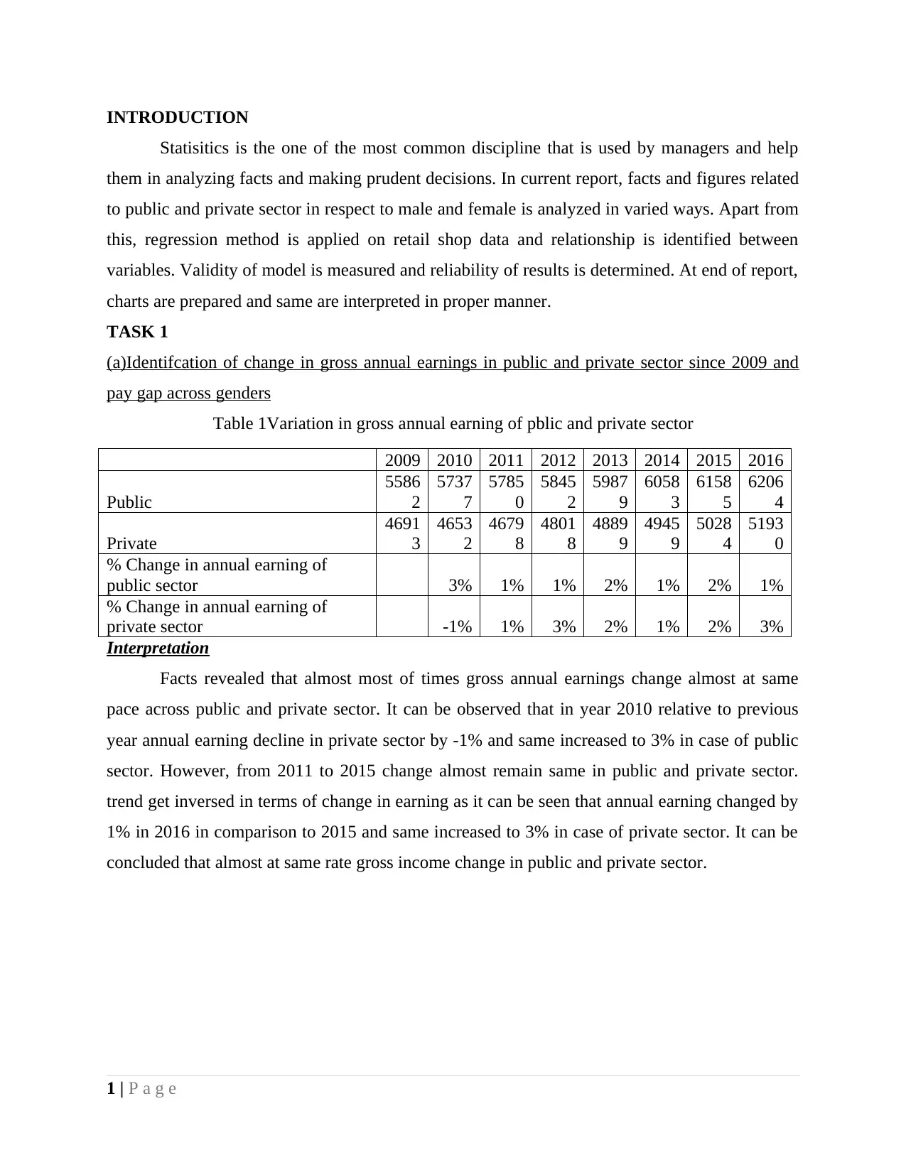
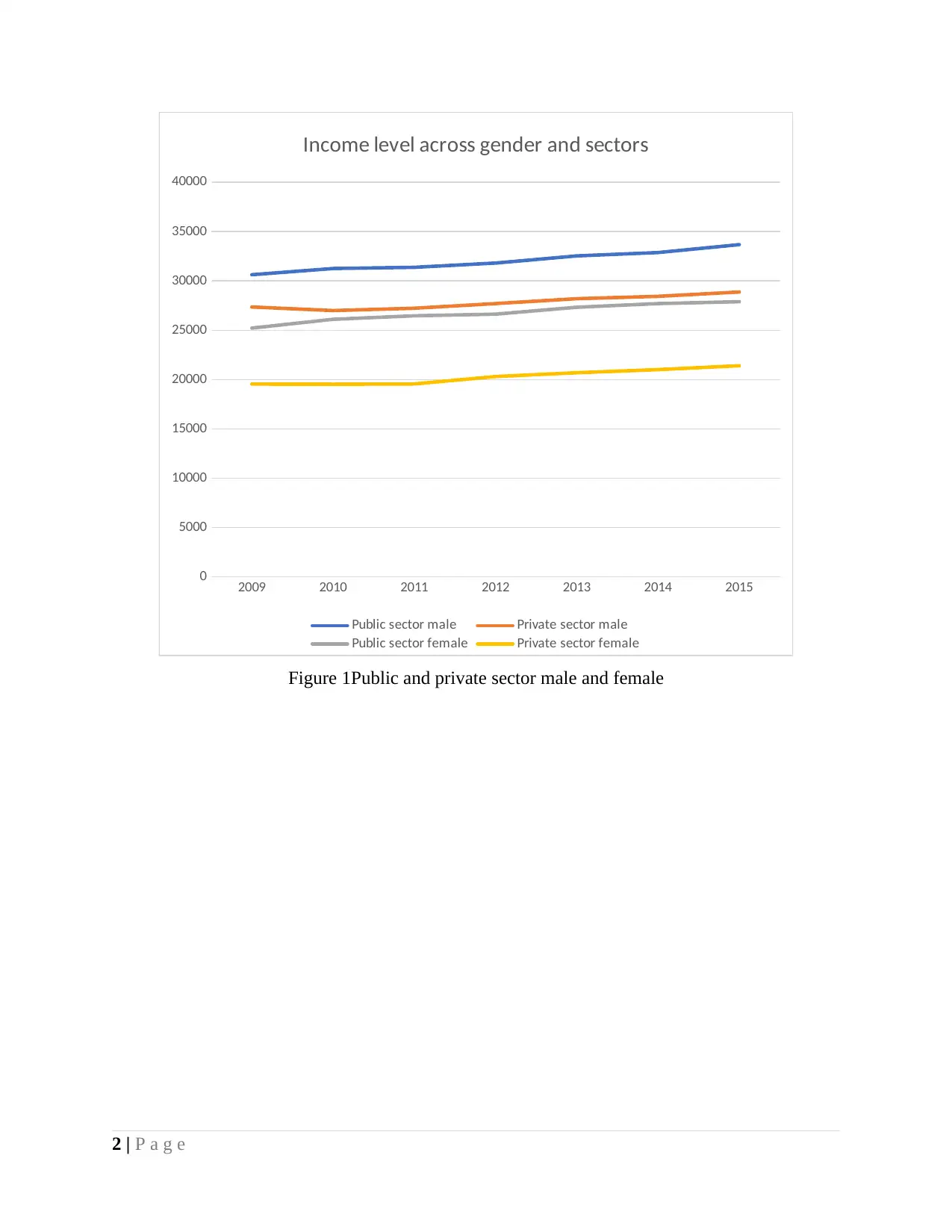
Interpretation
Facts revealed that almost most of times gross annual earnings change almost at same
pace across public and private sector. It can be observed that in year 2010 relative to previous
year annual earning decline in private sector by -1% and same increased to 3% in case of public
sector. However, from 2011 to 2015 change almost remain same in public and private sector.
trend get inversed in terms of change in earning as it can be seen that annual earning changed by
1% in 2016 in comparison to 2015 and same increased to 3% in case of private sector. It can be
concluded that almost at same rate gross income change in public and private sector.
1 | P a g e
Statisitics is the one of the most common discipline that is used by managers and help
them in analyzing facts and making prudent decisions. In current report, facts and figures related
to public and private sector in respect to male and female is analyzed in varied ways. Apart from
this, regression method is applied on retail shop data and relationship is identified between
variables. Validity of model is measured and reliability of results is determined. At end of report,
charts are prepared and same are interpreted in proper manner.
TASK 1
(a)Identifcation of change in gross annual earnings in public and private sector since 2009 and
pay gap across genders
Table 1Variation in gross annual earning of pblic and private sector
2009 2010 2011 2012 2013 2014 2015 2016
Public
5586
2
5737
7
5785
0
5845
2
5987
9
6058
3
6158
5
6206
4
Private
4691
3
4653
2
4679
8
4801
8
4889
9
4945
9
5028
4
5193
0
% Change in annual earning of
public sector 3% 1% 1% 2% 1% 2% 1%
% Change in annual earning of
private sector -1% 1% 3% 2% 1% 2% 3%
Interpretation
Facts revealed that almost most of times gross annual earnings change almost at same
pace across public and private sector. It can be observed that in year 2010 relative to previous
year annual earning decline in private sector by -1% and same increased to 3% in case of public
sector. However, from 2011 to 2015 change almost remain same in public and private sector.
trend get inversed in terms of change in earning as it can be seen that annual earning changed by
1% in 2016 in comparison to 2015 and same increased to 3% in case of private sector. It can be
concluded that almost at same rate gross income change in public and private sector.
1 | P a g e
Paraphrase This Document
Need a fresh take? Get an instant paraphrase of this document with our AI Paraphraser
2009 2010 2011 2012 2013 2014 2015
0
5000
10000
15000
20000
25000
30000
35000
40000
Income level across gender and sectors
Public sector male Private sector male
Public sector female Private sector female
Figure 1Public and private sector male and female
2 | P a g e
0
5000
10000
15000
20000
25000
30000
35000
40000
Income level across gender and sectors
Public sector male Private sector male
Public sector female Private sector female
Figure 1Public and private sector male and female
2 | P a g e
2009 2010 2011 2012 2013 2014 2015
0
5000
10000
15000
20000
25000
30000
35000
40000
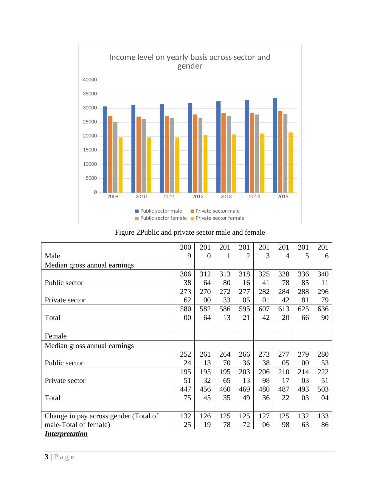
Income level on yearly basis across sector and
gender
Public sector male Private sector male
Public sector female Private sector female
Figure 2Public and private sector male and female
Male
200
9
201
0
201
1
201
2
201
3
201
4
201
5
201
6
Median gross annual earnings
Public sector
306
38
312
64
313
80
318
16
325
41
328
78
336
85
340
11
Private sector
273
62
270
00
272
33
277
05
282
01
284
42
288
81
296
79
Total
580
00
582
64
586
13
595
21
607
42
613
20
625
66
636
90
Female
Median gross annual earnings
Public sector
252
24
261
13
264
70
266
36
273
38
277
05
279
00
280
53
Private sector
195
51
195
32
195
65
203
13
206
98
210
17
214
03
222
51
Total
447
75
456
45
460
35
469
49
480
36
487
22
493
03
503
04
Change in pay across gender (Total of
male-Total of female)
132
25
126
19
125
78
125
72
127
06
125
98
132
63
133
86
Interpretation
3 | P a g e
0
5000
10000
15000
20000
25000
30000
35000
40000
Income level on yearly basis across sector and
gender
Public sector male Private sector male
Public sector female Private sector female
Figure 2Public and private sector male and female
Male
200
9
201
0
201
1
201
2
201
3
201
4
201
5
201
6
Median gross annual earnings
Public sector
306
38
312
64
313
80
318
16
325
41
328
78
336
85
340
11
Private sector
273
62
270
00
272
33
277
05
282
01
284
42
288
81
296
79
Total
580
00
582
64
586
13
595
21
607
42
613
20
625
66
636
90
Female
Median gross annual earnings
Public sector
252
24
261
13
264
70
266
36
273
38
277
05
279
00
280
53
Private sector
195
51
195
32
195
65
203
13
206
98
210
17
214
03
222
51
Total
447
75
456
45
460
35
469
49
480
36
487
22
493
03
503
04
Change in pay across gender (Total of
male-Total of female)
132
25
126
19
125
78
125
72
127
06
125
98
132
63
133
86
Interpretation
3 | P a g e
⊘ This is a preview!⊘
Do you want full access?
Subscribe today to unlock all pages.
Trusted by 1+ million students worldwide
Most of years it is observed that change in gender pay gap reduce which means that gap
that exist between male and female reduced in past couple of years consistently. However, in
year 2015 and 2016 this change get increased at rapid rate which is not good. hence, it can be
said that government need to handle entire situation because by doing so such kind of situations
can be controlled and prevented from occurance.
TASK 2
(a)Ogive chart and computation of mean as well as standard deviation
(1)
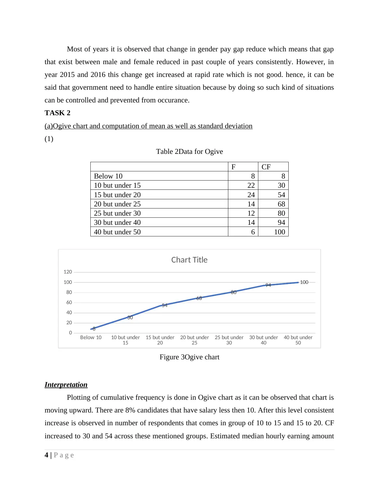
Table 2Data for Ogive
F CF
Below 10 8 8
10 but under 15 22 30
15 but under 20 24 54
20 but under 25 14 68
25 but under 30 12 80
30 but under 40 14 94
40 but under 50 6 100
Below 10 10 but under
15 15 but under
20 20 but under
25 25 but under
30 30 but under
40 40 but under
50
0
20
40
60
80
100
120
8
30
54
68
80
94 100
Chart Title
Figure 3Ogive chart
Interpretation
Plotting of cumulative frequency is done in Ogive chart as it can be observed that chart is
moving upward. There are 8% candidates that have salary less then 10. After this level consistent
increase is observed in number of respondents that comes in group of 10 to 15 and 15 to 20. CF
increased to 30 and 54 across these mentioned groups. Estimated median hourly earning amount
4 | P a g e
that exist between male and female reduced in past couple of years consistently. However, in
year 2015 and 2016 this change get increased at rapid rate which is not good. hence, it can be
said that government need to handle entire situation because by doing so such kind of situations
can be controlled and prevented from occurance.
TASK 2
(a)Ogive chart and computation of mean as well as standard deviation
(1)
Table 2Data for Ogive
F CF
Below 10 8 8
10 but under 15 22 30
15 but under 20 24 54
20 but under 25 14 68
25 but under 30 12 80
30 but under 40 14 94
40 but under 50 6 100
Below 10 10 but under
15 15 but under
20 20 but under
25 25 but under
30 30 but under
40 40 but under
50
0
20
40
60
80
100
120
8
30
54
68
80
94 100
Chart Title
Figure 3Ogive chart
Interpretation
Plotting of cumulative frequency is done in Ogive chart as it can be observed that chart is
moving upward. There are 8% candidates that have salary less then 10. After this level consistent
increase is observed in number of respondents that comes in group of 10 to 15 and 15 to 20. CF
increased to 30 and 54 across these mentioned groups. Estimated median hourly earning amount
4 | P a g e
Paraphrase This Document
Need a fresh take? Get an instant paraphrase of this document with our AI Paraphraser
is 14 because above this number there are three observations and below this number there are
three observations. Hence, due to this reason range 20 to 25 is considered as median range.
Quartile value at 0.50 and median value is same. Range below10 comes in first quartile and in
third quartile range 25 to 30 may come. In last and final quartile 30 to 40 category comes. In this
way, entire data is distributed in different quartiles.
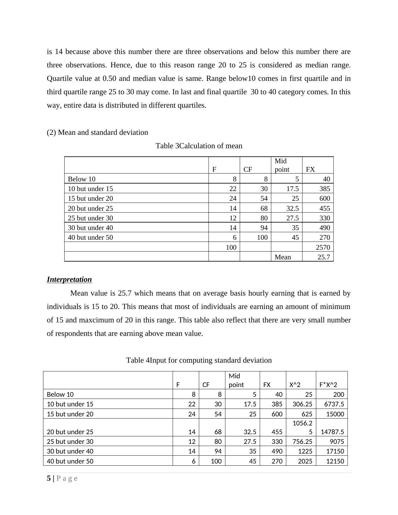
(2) Mean and standard deviation
Table 3Calculation of mean
F CF
Mid
point FX
Below 10 8 8 5 40
10 but under 15 22 30 17.5 385
15 but under 20 24 54 25 600
20 but under 25 14 68 32.5 455
25 but under 30 12 80 27.5 330
30 but under 40 14 94 35 490
40 but under 50 6 100 45 270
100 2570
Mean 25.7
Interpretation
Mean value is 25.7 which means that on average basis hourly earning that is earned by
individuals is 15 to 20. This means that most of individuals are earning an amount of minimum
of 15 and maxcimum of 20 in this range. This table also reflect that there are very small number
of respondents that are earning above mean value.
Table 4Input for computing standard deviation
F CF
Mid
point FX X^2 F*X^2
Below 10 8 8 5 40 25 200
10 but under 15 22 30 17.5 385 306.25 6737.5
15 but under 20 24 54 25 600 625 15000
20 but under 25 14 68 32.5 455
1056.2
5 14787.5
25 but under 30 12 80 27.5 330 756.25 9075
30 but under 40 14 94 35 490 1225 17150
40 but under 50 6 100 45 270 2025 12150
5 | P a g e
three observations. Hence, due to this reason range 20 to 25 is considered as median range.
Quartile value at 0.50 and median value is same. Range below10 comes in first quartile and in
third quartile range 25 to 30 may come. In last and final quartile 30 to 40 category comes. In this
way, entire data is distributed in different quartiles.
(2) Mean and standard deviation
Table 3Calculation of mean
F CF
Mid
point FX
Below 10 8 8 5 40
10 but under 15 22 30 17.5 385
15 but under 20 24 54 25 600
20 but under 25 14 68 32.5 455
25 but under 30 12 80 27.5 330
30 but under 40 14 94 35 490
40 but under 50 6 100 45 270
100 2570
Mean 25.7
Interpretation
Mean value is 25.7 which means that on average basis hourly earning that is earned by
individuals is 15 to 20. This means that most of individuals are earning an amount of minimum
of 15 and maxcimum of 20 in this range. This table also reflect that there are very small number
of respondents that are earning above mean value.
Table 4Input for computing standard deviation
F CF
Mid
point FX X^2 F*X^2
Below 10 8 8 5 40 25 200
10 but under 15 22 30 17.5 385 306.25 6737.5
15 but under 20 24 54 25 600 625 15000
20 but under 25 14 68 32.5 455
1056.2
5 14787.5
25 but under 30 12 80 27.5 330 756.25 9075
30 but under 40 14 94 35 490 1225 17150
40 but under 50 6 100 45 270 2025 12150
5 | P a g e
100 2570
660490
0
Mean 25.7 660.49
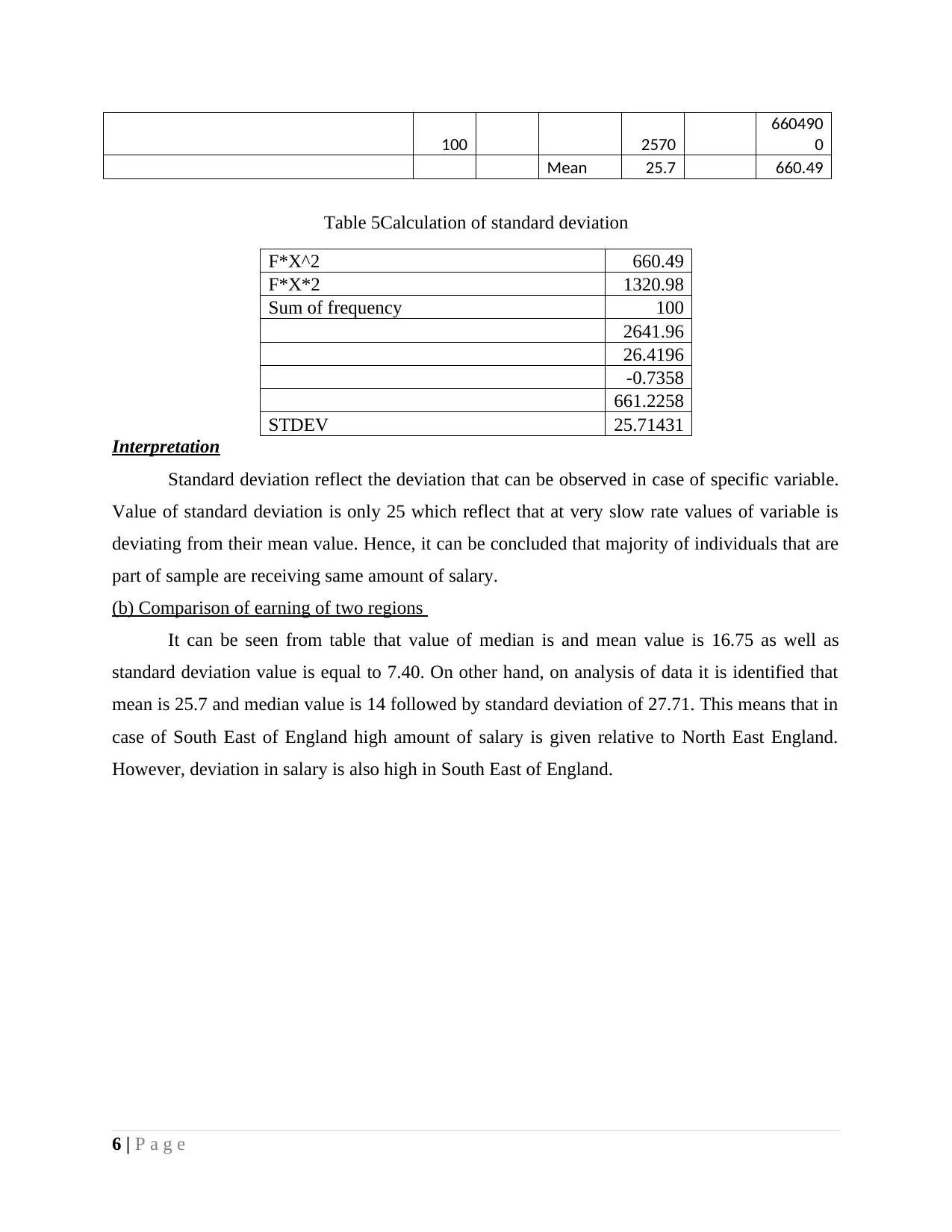
Table 5Calculation of standard deviation
F*X^2 660.49
F*X*2 1320.98
Sum of frequency 100
2641.96
26.4196
-0.7358
661.2258
STDEV 25.71431
Interpretation
Standard deviation reflect the deviation that can be observed in case of specific variable.
Value of standard deviation is only 25 which reflect that at very slow rate values of variable is
deviating from their mean value. Hence, it can be concluded that majority of individuals that are
part of sample are receiving same amount of salary.
(b) Comparison of earning of two regions
It can be seen from table that value of median is and mean value is 16.75 as well as
standard deviation value is equal to 7.40. On other hand, on analysis of data it is identified that
mean is 25.7 and median value is 14 followed by standard deviation of 27.71. This means that in
case of South East of England high amount of salary is given relative to North East England.
However, deviation in salary is also high in South East of England.
6 | P a g e
660490
0
Mean 25.7 660.49
Table 5Calculation of standard deviation
F*X^2 660.49
F*X*2 1320.98
Sum of frequency 100
2641.96
26.4196
-0.7358
661.2258
STDEV 25.71431
Interpretation
Standard deviation reflect the deviation that can be observed in case of specific variable.
Value of standard deviation is only 25 which reflect that at very slow rate values of variable is
deviating from their mean value. Hence, it can be concluded that majority of individuals that are
part of sample are receiving same amount of salary.
(b) Comparison of earning of two regions
It can be seen from table that value of median is and mean value is 16.75 as well as
standard deviation value is equal to 7.40. On other hand, on analysis of data it is identified that
mean is 25.7 and median value is 14 followed by standard deviation of 27.71. This means that in
case of South East of England high amount of salary is given relative to North East England.
However, deviation in salary is also high in South East of England.
6 | P a g e
⊘ This is a preview!⊘
Do you want full access?
Subscribe today to unlock all pages.
Trusted by 1+ million students worldwide
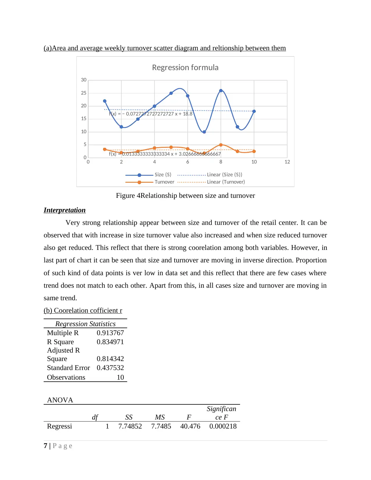
(a)Area and average weekly turnover scatter diagram and reltionship between them
0 2 4 6 8 10 12
0
5
10
15
20
25
30
f(x) = 0.0133333333333334 x + 3.02666666666667
f(x) = − 0.0727272727272727 x + 18.8
Regression formula
Size (S) Linear (Size (S))
Turnover Linear (Turnover)
Figure 4Relationship between size and turnover
Interpretation
Very strong relationship appear between size and turnover of the retail center. It can be
observed that with increase in size turnover value also increased and when size reduced turnover
also get reduced. This reflect that there is strong coorelation among both variables. However, in
last part of chart it can be seen that size and turnover are moving in inverse direction. Proportion
of such kind of data points is ver low in data set and this reflect that there are few cases where
trend does not match to each other. Apart from this, in all cases size and turnover are moving in
same trend.
(b) Coorelation cofficient r
Regression Statistics
Multiple R 0.913767
R Square 0.834971
Adjusted R
Square 0.814342
Standard Error 0.437532
Observations 10
ANOVA
df SS MS F
Significan
ce F
Regressi 1 7.74852 7.7485 40.476 0.000218
7 | P a g e
Paraphrase This Document
Need a fresh take? Get an instant paraphrase of this document with our AI Paraphraser
on 8 28 22
Residual 8
1.53147
2
0.1914
34
Total 9 9.28
Coefficie
nts
Standar
d Error t Stat
P-
value
Lower
95%
Upper
95%
Lower
95.0%
Upper
95.0%
Intercept 0.202177
0.47603
4
0.4247
11
0.6822
39 -0.89556
1.2999
12
-
0.8955
6
1.2999
12
Size (S) 0.15749
0.02475
4
6.3620
93
0.0002
18 0.100406
0.2145
74
0.1004
06
0.2145
74
RESIDUAL OUTPUT
Observati
on
Predicted
Turnover
Residua
ls
1 3.666965
-
0.36697
2 2.092061
-
0.09206
3 2.564533
-
0.06453
4 3.351985
0.44801
5
5 4.139437
-
0.03944
6 3.981946
-
0.48195
7 1.777081
0.02291
9
8 4.296927
0.70307
3
9 2.092061
0.40793
9
10 3.037004 -0.537
PROBABILITY
OUTPUT
Percent
ile
Turnov
er
5 1.8
15 2
8 | P a g e
25 2.5
35 2.5
45 2.5
55 3.3
65 3.5
75 3.8
85 4.1
95 5
8 10 12 14 16 18 20 22 24 26 28
0
1
2
3
4
5
6
3.3
2 2.5
3.8 4.1
3.5
1.8
5
2.5 2.5
Size (S) Line Fit Plot
Turnover
Predicted Turnover
Size (S)
Turnover
0 10 20 30 40 50 60 70 80 90 100
0
2
4
6
Normal Probability Plot
Sample Percentile
Turnover
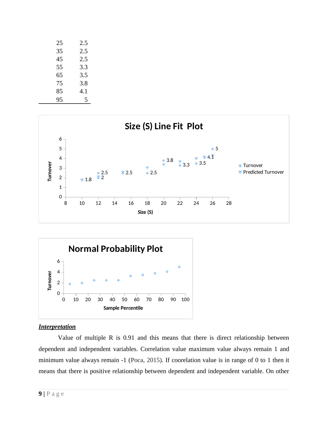
Interpretation
Value of multiple R is 0.91 and this means that there is direct relationship between
dependent and independent variables. Correlation value maximum value always remain 1 and
minimum value always remain -1 (Poca, 2015). If coorelation value is in range of 0 to 1 then it
means that there is positive relationship between dependent and independent variable. On other
9 | P a g e
35 2.5
45 2.5
55 3.3
65 3.5
75 3.8
85 4.1
95 5
8 10 12 14 16 18 20 22 24 26 28
0
1
2
3
4
5
6
3.3
2 2.5
3.8 4.1
3.5
1.8
5
2.5 2.5
Size (S) Line Fit Plot
Turnover
Predicted Turnover
Size (S)
Turnover
0 10 20 30 40 50 60 70 80 90 100
0
2
4
6
Normal Probability Plot
Sample Percentile
Turnover
Interpretation
Value of multiple R is 0.91 and this means that there is direct relationship between
dependent and independent variables. Correlation value maximum value always remain 1 and
minimum value always remain -1 (Poca, 2015). If coorelation value is in range of 0 to 1 then it
means that there is positive relationship between dependent and independent variable. On other
9 | P a g e
⊘ This is a preview!⊘
Do you want full access?
Subscribe today to unlock all pages.
Trusted by 1+ million students worldwide
1 out of 19
Related Documents


Your All-in-One AI-Powered Toolkit for Academic Success.
+13062052269
info@desklib.com
Available 24*7 on WhatsApp / Email
![[object Object]](/_next/static/media/star-bottom.7253800d.svg)
Unlock your academic potential
Copyright © 2020–2026 A2Z Services. All Rights Reserved. Developed and managed by ZUCOL.