Statistical Analysis Report: Earnings, Turnover, and Delivery Data

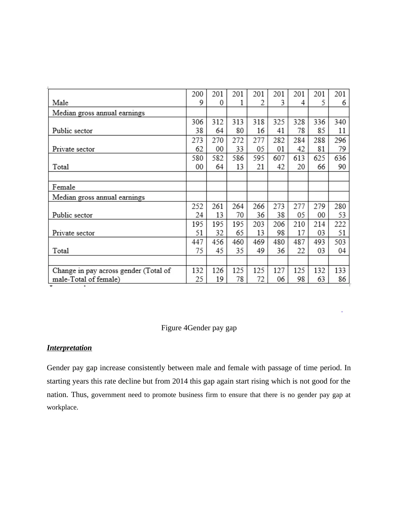
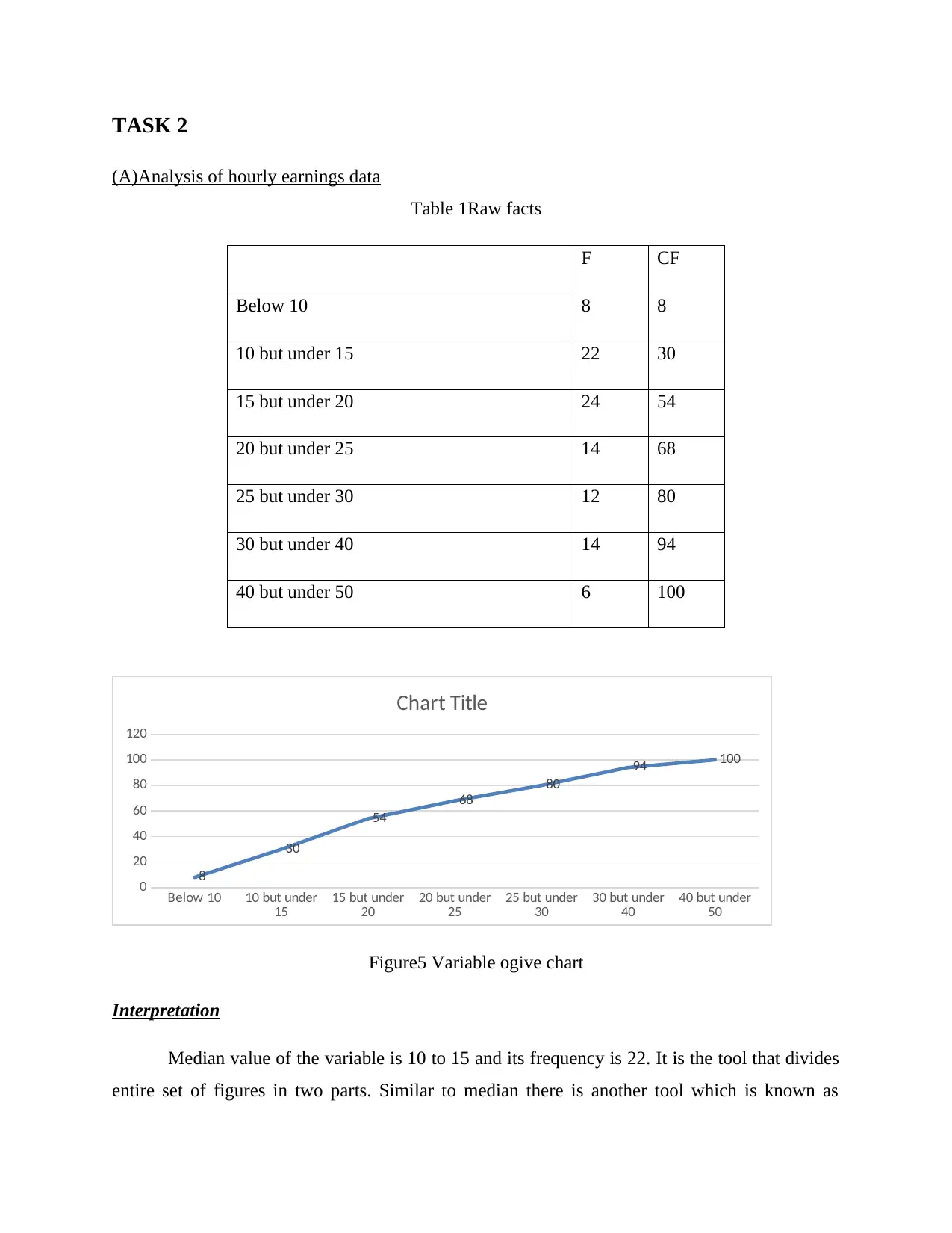
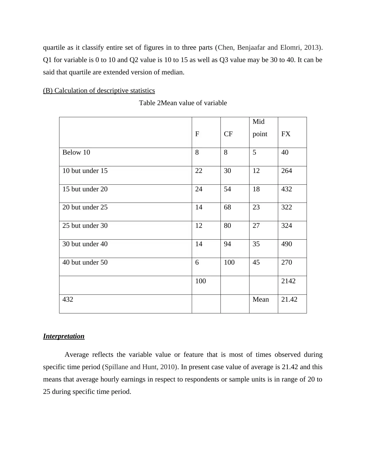
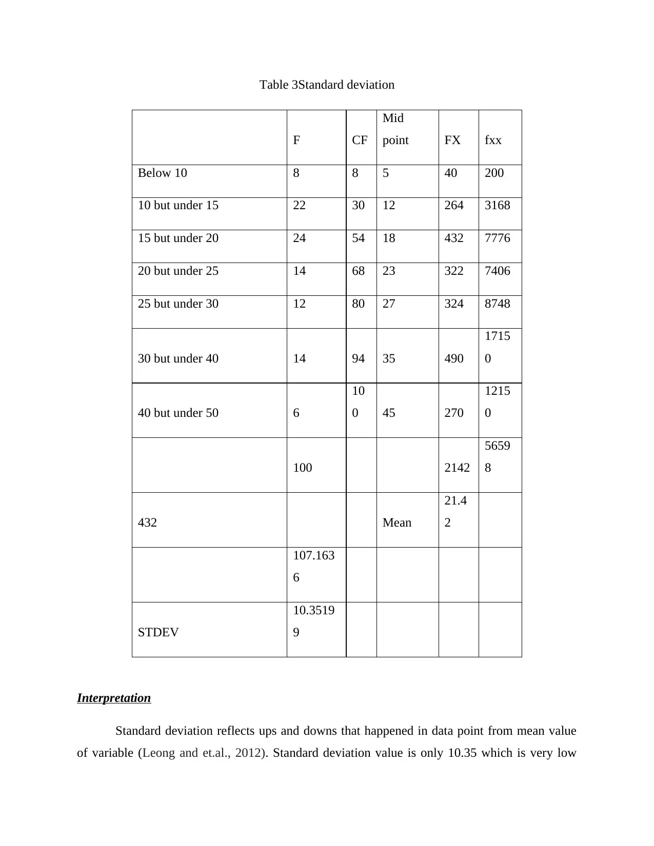
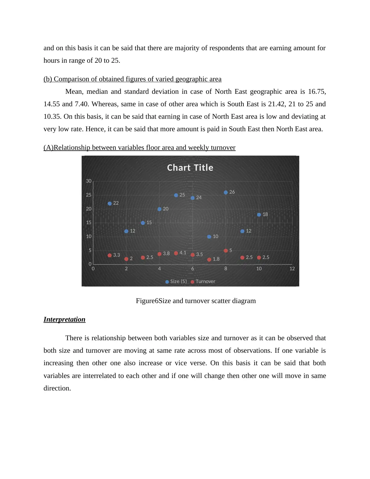
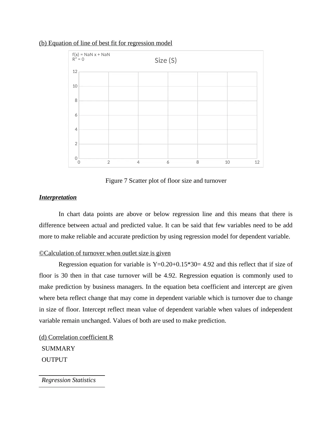
This report presents a comprehensive statistical analysis of various datasets. The study begins with an examination of earnings in both public and private sectors, along with a gender pay gap analysis. It then delves into hourly earnings data, calculating descriptive statistics such as mean, median, and standard deviation, and comparing figures across geographic areas. Regression analysis is applied to floor area and weekly turnover data to determine relationships and predict outcomes. Furthermore, the report investigates delivery patterns, calculating the economic order quantity (EOQ) and comparing it to associated costs. The analysis incorporates scatter diagrams, line charts, and ogive charts to visualize the data and facilitate interpretation. The report concludes by summarizing the key findings and highlighting the significance of statistical tools in business decision-making.

STATISTICS

TABLE OF CONTENTS
INTRODUCTION.......................................................................................................................................3
TASK 1.......................................................................................................................................................3
(a)Change in gross annual earning in public and private sector and pay gap across gender....................3
TASK 2.......................................................................................................................................................6
(A)Analysis of hourly earnings data........................................................................................................6
(B) Calculation of descriptive statistics...................................................................................................7
(b) Comparison of obtained figures of varied geographic area................................................................8
(A)Relationship between variables floor area and weekly turnover.........................................................9
(b) Equation of line of best fit for regression model..............................................................................10
©Calculation of turnover when outlet size is given...............................................................................10
(d) Correlation coefficient R..................................................................................................................10
(e) Measuring statistical validity of model.............................................................................................13
TASK 3.....................................................................................................................................................14
(a)Number of delivery made on annual basis.........................................................................................14
(b) Deliveries made on each round........................................................................................................14
©Economic order quantity.....................................................................................................................14
(d) Comparison of EOQ and cost...........................................................................................................15
TASK 4.....................................................................................................................................................15
(a)Scatter diagram of size and turnover.................................................................................................15
(b)Male income level line chart.............................................................................................................17
©Ogive chart for computing cumulative percentage of employees for hourly earnings data.................18
CONCLUSION.........................................................................................................................................19
REFERENCES..........................................................................................................................................20

INTRODUCTION
Statistics is the one of the most important branch that assist managers in making business
decisions and identifying factors due to which business performance is affected. In present
research study male and female earning data is analyzed deeply and charting of same is done.
Apart from this, regression analysis method is applied on size and turnover data set and
prediction is made about given value of independent variable. At end of the report charting of
variables is done and conclusion is formed.
TASK 1
(a)Change in gross annual earning in public and private sector and pay gap across gender
Figure 1Change in annual earning in public and private sector
Interpretation
Changes happened in public and private sector earning at same rate every year.
Fluctuation is observed consistently in the earning in both sectors as it change from 1% to 3%
every year. This reflects that every year 1% up and down usually happened in growth rate of
annual earning but in specific range these rates are changing.

2009 2010 2011 2012 2013 2014 2015
0
5000
10000
15000
20000
25000
30000
35000
40000
30638 31264 31380 31816 32541 32878 33685
27362 27000 27233 27705 28201 28442 28881
25224 26113 26470 26636 27338 27705 27900
19551 19532 19565 20313 20698 21017 21403
Chart Title
Public sector male Private sector male
Public sector female Private sector female
Figure2Public and private sector male and female
2009 2010 2011 2012 2013 2014 2015
0
5000
10000
15000
20000
25000
30000
35000
40000
Chart Title
Public sector male Private sector male
Public sector female Private sector female
Figure3Public and private sector male and female

Figure 4Gender pay gap
Interpretation
Gender pay gap increase consistently between male and female with passage of time period. In
starting years this rate decline but from 2014 this gap again start rising which is not good for the
nation. Thus, government need to promote business firm to ensure that there is no gender pay gap at
workplace.

TASK 2
(A)Analysis of hourly earnings data
Table 1Raw facts
F CF
Below 10 8 8
10 but under 15 22 30
15 but under 20 24 54
20 but under 25 14 68
25 but under 30 12 80
30 but under 40 14 94
40 but under 50 6 100
Below 10 10 but under
15 15 but under
20 20 but under
25 25 but under
30 30 but under
40 40 but under
50
0
20
40
60
80
100
120
8
30
54
68
80
94 100
Chart Title
Figure5 Variable ogive chart
Interpretation
Median value of the variable is 10 to 15 and its frequency is 22. It is the tool that divides
entire set of figures in two parts. Similar to median there is another tool which is known as

quartile as it classify entire set of figures in to three parts (Chen, Benjaafar and Elomri, 2013).
Q1 for variable is 0 to 10 and Q2 value is 10 to 15 as well as Q3 value may be 30 to 40. It can be
said that quartile are extended version of median.
(B) Calculation of descriptive statistics
Table 2Mean value of variable
F CF
Mid
point FX
Below 10 8 8 5 40
10 but under 15 22 30 12 264
15 but under 20 24 54 18 432
20 but under 25 14 68 23 322
25 but under 30 12 80 27 324
30 but under 40 14 94 35 490
40 but under 50 6 100 45 270
100 2142
432 Mean 21.42
Interpretation
Average reflects the variable value or feature that is most of times observed during
specific time period (Spillane and Hunt, 2010). In present case value of average is 21.42 and this
means that average hourly earnings in respect to respondents or sample units is in range of 20 to
25 during specific time period.

Table 3Standard deviation
F CF
Mid
point FX fxx
Below 10 8 8 5 40 200
10 but under 15 22 30 12 264 3168
15 but under 20 24 54 18 432 7776
20 but under 25 14 68 23 322 7406
25 but under 30 12 80 27 324 8748
30 but under 40 14 94 35 490
1715
0
40 but under 50 6
10
0 45 270
1215
0
100 2142
5659
8
432 Mean
21.4
2
107.163
6
STDEV
10.3519
9
Interpretation
Standard deviation reflects ups and downs that happened in data point from mean value
of variable (Leong and et.al., 2012). Standard deviation value is only 10.35 which is very low

and on this basis it can be said that there are majority of respondents that are earning amount for
hours in range of 20 to 25.
(b) Comparison of obtained figures of varied geographic area
Mean, median and standard deviation in case of North East geographic area is 16.75,
14.55 and 7.40. Whereas, same in case of other area which is South East is 21.42, 21 to 25 and
10.35. On this basis, it can be said that earning in case of North East area is low and deviating at
very low rate. Hence, it can be said that more amount is paid in South East then North East area.
(A)Relationship between variables floor area and weekly turnover
0 2 4 6 8 10 12
0
5
10
15
20
25
30
3.3 2 2.5 3.8 4.1 3.5 1.8
5
2.5 2.5
22
12
15
20
25 24
10
26
12
18
Chart Title
Size (S) Turnover
Figure6Size and turnover scatter diagram
Interpretation
There is relationship between both variables size and turnover as it can be observed that
both size and turnover are moving at same rate across most of observations. If one variable is
increasing then other one also increase or vice verse. On this basis it can be said that both
variables are interrelated to each other and if one will change then other one will move in same
direction.

(b) Equation of line of best fit for regression model
0 2 4 6 8 10 12
0
2
4
6
8
10
12
f(x) = NaN x + NaN
R² = 0 Size (S)
Figure 7 Scatter plot of floor size and turnover
Interpretation
In chart data points are above or below regression line and this means that there is
difference between actual and predicted value. It can be said that few variables need to be add
more to make reliable and accurate prediction by using regression model for dependent variable.
©Calculation of turnover when outlet size is given
Regression equation for variable is Y=0.20+0.15*30= 4.92 and this reflect that if size of
floor is 30 then in that case turnover will be 4.92. Regression equation is commonly used to
make prediction by business managers. In the equation beta coefficient and intercept are given
where beta reflect change that may come in dependent variable which is turnover due to change
in size of floor. Intercept reflect mean value of dependent variable when values of independent
variable remain unchanged. Values of both are used to make prediction.
(d) Correlation coefficient R
SUMMARY
OUTPUT
Regression Statistics

Multiple R 0.913767
R Square 0.834971
Adjusted
R Square 0.814342
Standard
Error 0.437532
Observatio
ns 10
ANOVA
df SS MS F
Significan
ce F
Regressio
n 1
7.7485
28
7.7485
28
40.476
22 0.000218
Residual 8
1.5314
72
0.1914
34
Total 9 9.28
Coefficie
nts
Standar
d Error t Stat P-value
Lower
95%
Upper
95%
Lower
95.0%
Upper
95.0%
Intercept 0.202177
0.4760
34
0.4247
11
0.6822
39 -0.89556
1.2999
12
-
0.8955
6
1.2999
12
Size (S) 0.15749
0.0247
54
6.3620
93
0.0002
18 0.100406
0.2145
74
0.1004
06
0.2145
74
RESIDUAL OUTPUT
Observati
on
Predicted
Turnover
Residua
ls
Standar
d
Residua

ls
1 3.666965
-
0.3669
7
-
0.8895
9
2 2.092061
-
0.0920
6
-
0.2231
7
3 2.564533
-
0.0645
3
-
0.1564
4
4 3.351985
0.4480
15
1.0860
74
5 4.139437
-
0.0394
4 -0.0956
6 3.981946
-
0.4819
5
-
1.1683
3
7 1.777081
0.0229
19
0.0555
61
8 4.296927
0.7030
73
1.7043
83
9 2.092061
0.4079
39
0.9889
21
10 3.037004 -0.537 -1.3018