Statistics: Decision Making, Hotel Modeling, Regression Analysis
VerifiedAdded on 2021/06/17
|29
|2341
|5
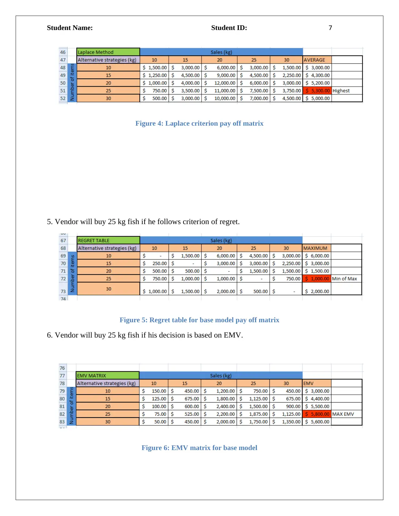
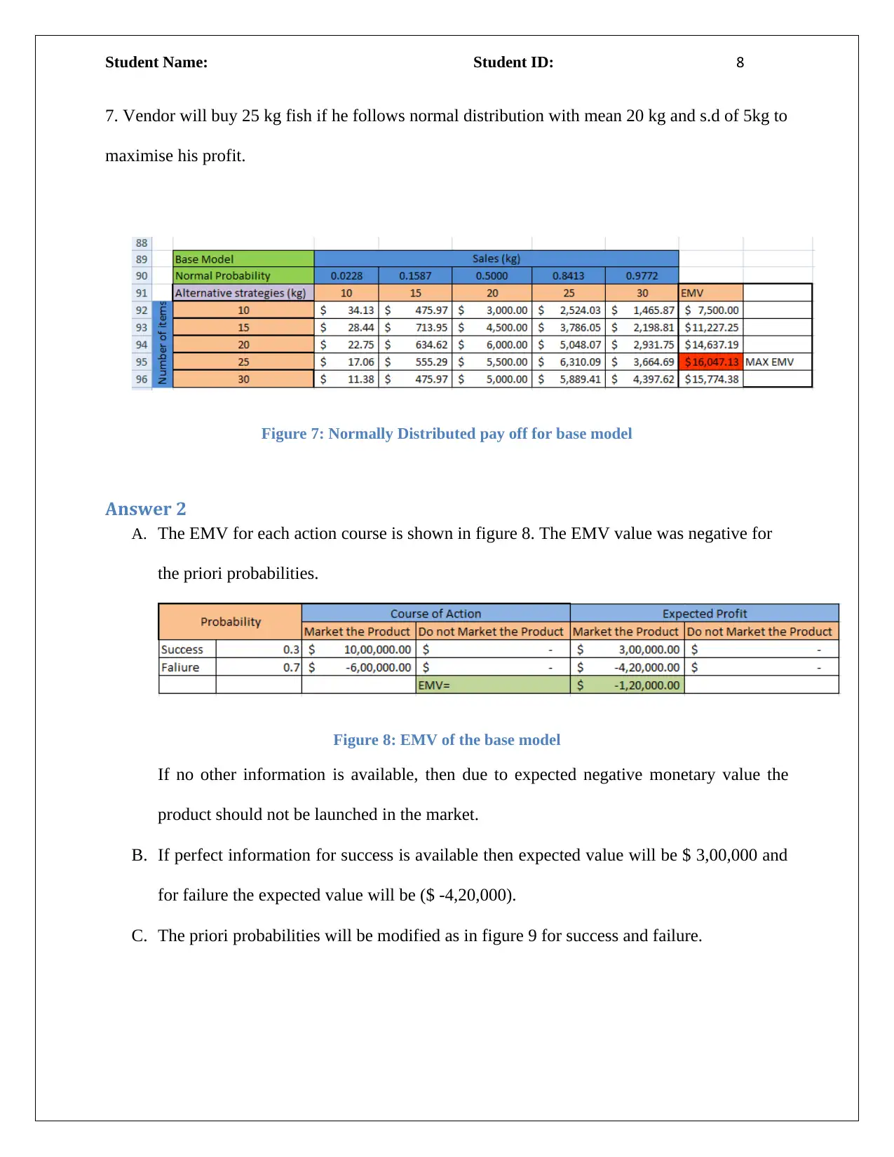
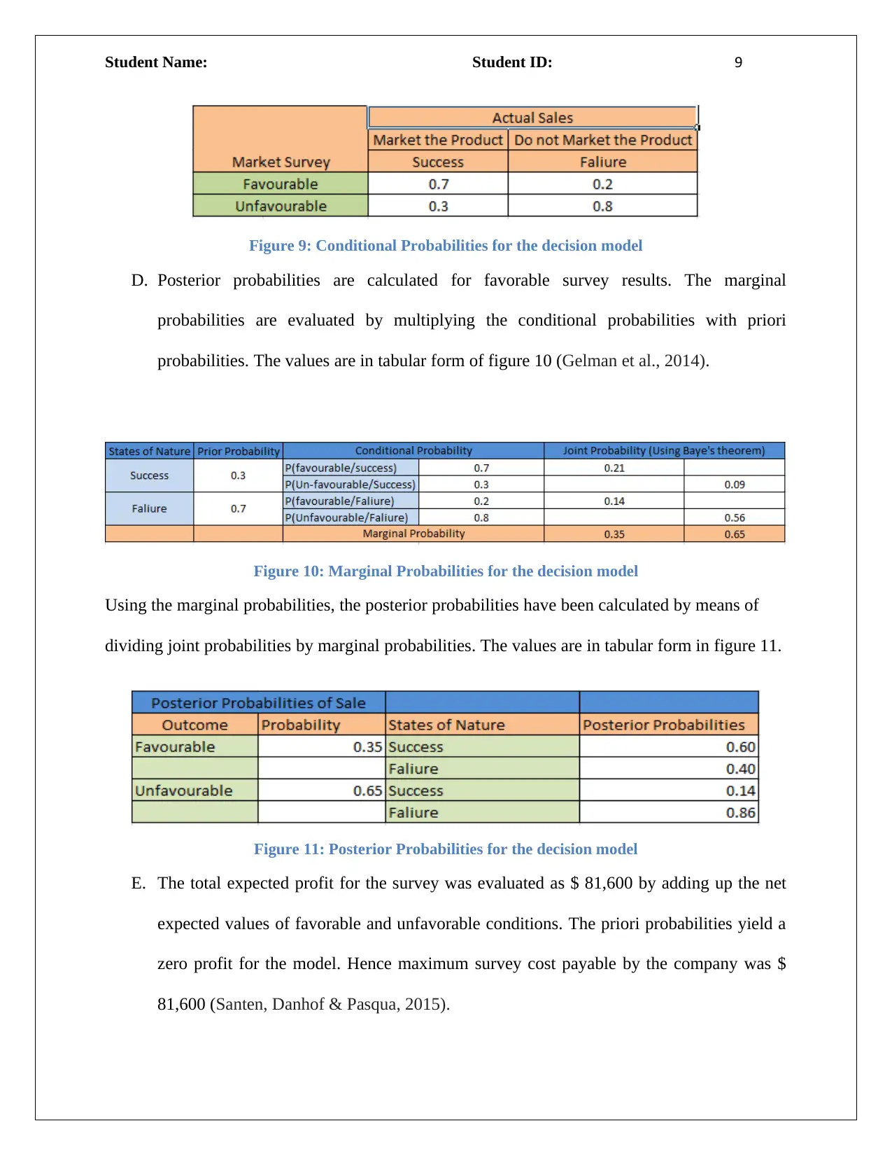
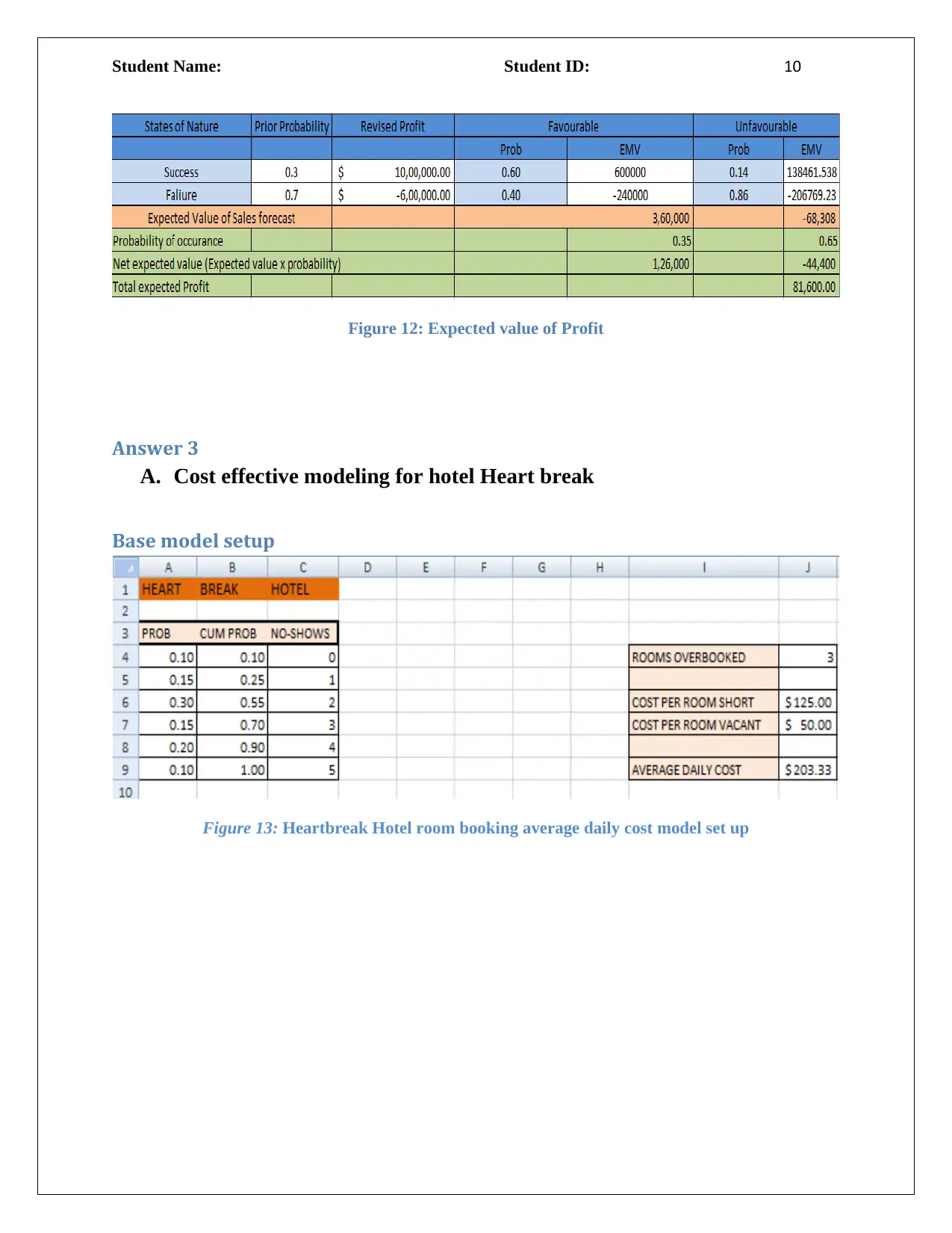
Homework Assignment
AI Summary
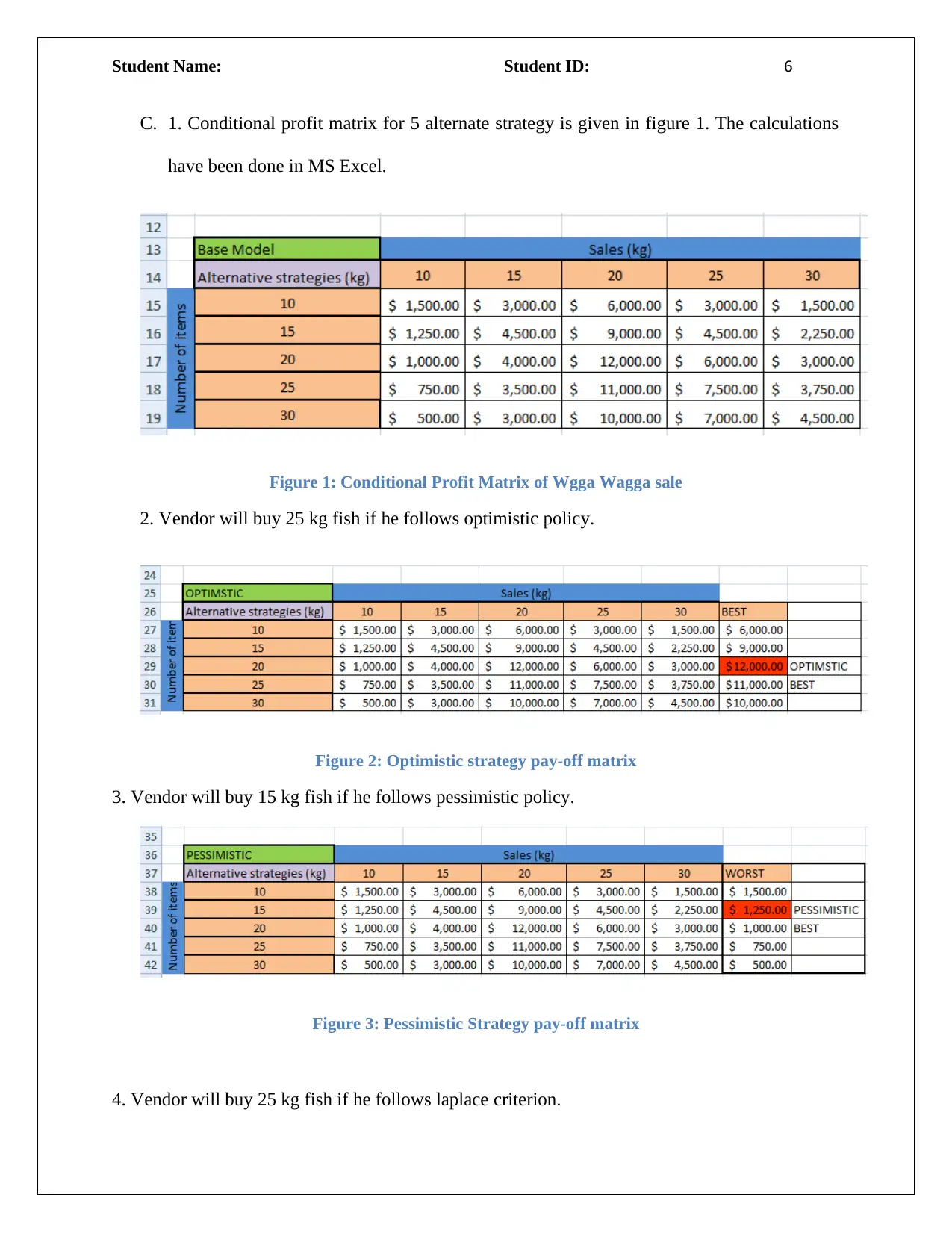
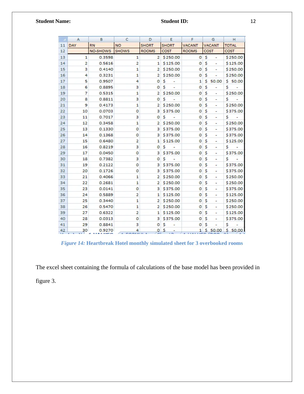
This assignment presents a detailed analysis of statistical concepts through various problem-solving scenarios. It begins with an exploration of decision-making processes, including the use of conditional profit matrices, optimistic and pessimistic strategies, Laplace criterion, and EMV (Expected Monetary Value) analysis to determine optimal choices. The assignment then delves into cost-effective modeling for a hotel, simulating room bookings, analyzing overbooking scenarios, and providing suggestions to the hotel manager. Furthermore, it investigates regression models to assess the relationship between car prices and factors like mileage and age, including the evaluation of correlation between variables. Finally, the assignment concludes with model setup and solver solutions using MS Excel to determine optimal profit levels for different products.


1 out of 29
Related Documents


![Accounting Decision Support Tools Assessment Item 3 Solution [Date]](/_next/image/?url=https%3A%2F%2Fdesklib.com%2Fmedia%2Fimages%2Fwx%2F8b0579db5dc54829a8e805e0dcb6f432.jpg&w=256&q=75)
![Assignment: Accounting Decision Support Tools - [Date] - Finance](/_next/image/?url=https%3A%2F%2Fdesklib.com%2Fmedia%2Fimages%2Fga%2F85e3fe63d61d4af3a506409b3f137201.jpg&w=256&q=75)
Your All-in-One AI-Powered Toolkit for Academic Success.
+13062052269
info@desklib.com
Available 24*7 on WhatsApp / Email
![[object Object]](/_next/static/media/star-bottom.7253800d.svg)
Copyright © 2020–2026 A2Z Services. All Rights Reserved. Developed and managed by ZUCOL.