Statistics Homework: Descriptive and Inferential Analysis, Sept 2018

This assignment provides solutions to a statistics homework problem involving descriptive and inferential statistical analysis. The descriptive statistics section calculates means, percentages, and generates a depression score, addressing missing data and outlier detection using SPSS. The inferential statistics section includes a paired t-test to compare pre- and post-treatment scores, revealing a significant improvement in PTSD symptoms. Additionally, ANOVA tests are conducted to compare groups and assess the impact of a long-term intervention on PSTD scores, demonstrating a statistically significant reduction over time. The analysis incorporates APA formatting for reporting results and discusses the assumptions and corrections applied in the repeated measures ANOVA. Desklib offers a wide range of study resources, including past papers and solved assignments, to support students in their academic endeavors.

Statistics
Student Name:
Instructor Name:
Course Number:
2 September 2018

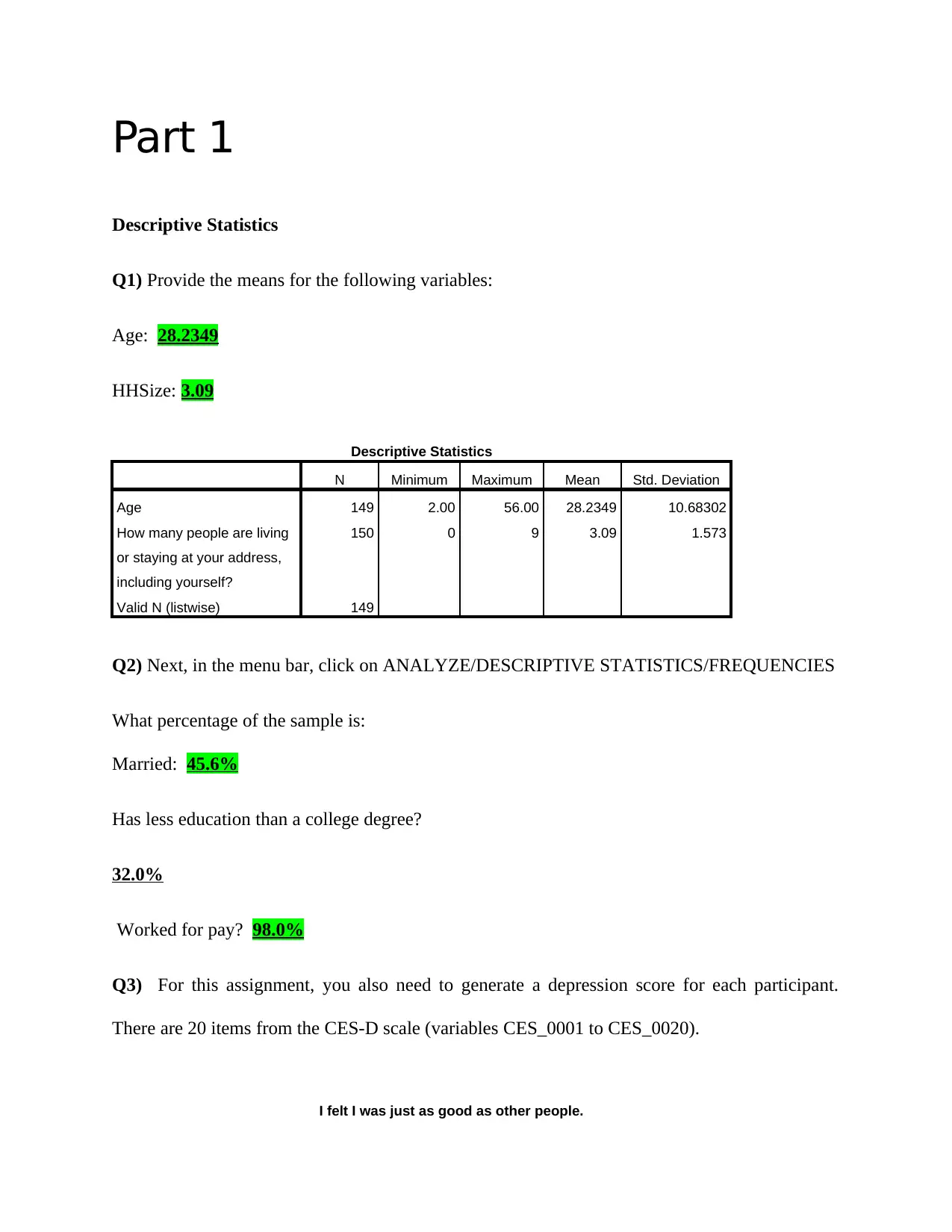
Part 1
Descriptive Statistics
Q1) Provide the means for the following variables:
Age: 28.2349
HHSize: 3.09
Descriptive Statistics
N Minimum Maximum Mean Std. Deviation
Age 149 2.00 56.00 28.2349 10.68302
How many people are living
or staying at your address,
including yourself?
150 0 9 3.09 1.573
Valid N (listwise) 149
Q2) Next, in the menu bar, click on ANALYZE/DESCRIPTIVE STATISTICS/FREQUENCIES
What percentage of the sample is:
Married: 45.6%
Has less education than a college degree?
32.0%
Worked for pay? 98.0%
Q3) For this assignment, you also need to generate a depression score for each participant.
There are 20 items from the CES-D scale (variables CES_0001 to CES_0020).
I felt I was just as good as other people.

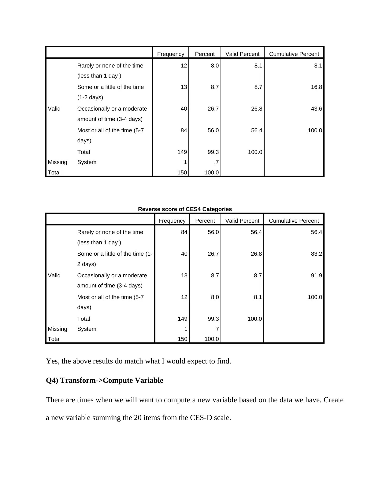
Frequency Percent Valid Percent Cumulative Percent
Valid
Rarely or none of the time
(less than 1 day )
12 8.0 8.1 8.1
Some or a little of the time
(1-2 days)
13 8.7 8.7 16.8
Occasionally or a moderate
amount of time (3-4 days)
40 26.7 26.8 43.6
Most or all of the time (5-7
days)
84 56.0 56.4 100.0
Total 149 99.3 100.0
Missing System 1 .7
Total 150 100.0
Reverse score of CES4 Categories
Frequency Percent Valid Percent Cumulative Percent
Valid
Rarely or none of the time
(less than 1 day )
84 56.0 56.4 56.4
Some or a little of the time (1-
2 days)
40 26.7 26.8 83.2
Occasionally or a moderate
amount of time (3-4 days)
13 8.7 8.7 91.9
Most or all of the time (5-7
days)
12 8.0 8.1 100.0
Total 149 99.3 100.0
Missing System 1 .7
Total 150 100.0
Yes, the above results do match what I would expect to find.
Q4) Transform->Compute Variable
There are times when we will want to compute a new variable based on the data we have. Create
a new variable summing the 20 items from the CES-D scale.

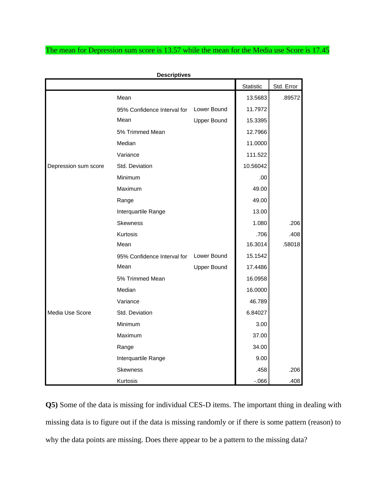
The mean for Depression sum score is 13.57 while the mean for the Media use Score is 17.45
Descriptives
Statistic Std. Error
Depression sum score
Mean 13.5683 .89572
95% Confidence Interval for
Mean
Lower Bound 11.7972
Upper Bound 15.3395
5% Trimmed Mean 12.7966
Median 11.0000
Variance 111.522
Std. Deviation 10.56042
Minimum .00
Maximum 49.00
Range 49.00
Interquartile Range 13.00
Skewness 1.080 .206
Kurtosis .706 .408
Media Use Score
Mean 16.3014 .58018
95% Confidence Interval for
Mean
Lower Bound 15.1542
Upper Bound 17.4486
5% Trimmed Mean 16.0958
Median 16.0000
Variance 46.789
Std. Deviation 6.84027
Minimum 3.00
Maximum 37.00
Range 34.00
Interquartile Range 9.00
Skewness .458 .206
Kurtosis -.066 .408
Q5) Some of the data is missing for individual CES-D items. The important thing in dealing with
missing data is to figure out if the data is missing randomly or if there is some pattern (reason) to
why the data points are missing. Does there appear to be a pattern to the missing data?

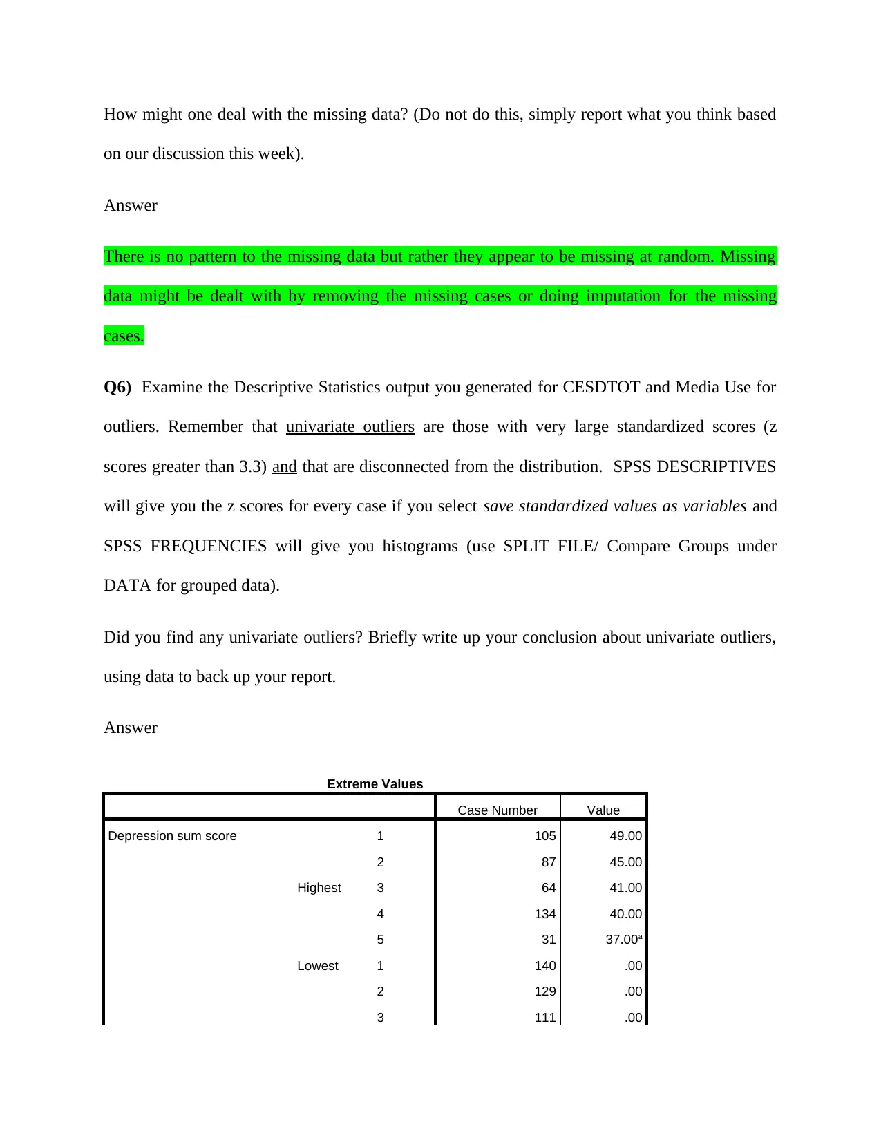
How might one deal with the missing data? (Do not do this, simply report what you think based
on our discussion this week).
Answer
There is no pattern to the missing data but rather they appear to be missing at random. Missing
data might be dealt with by removing the missing cases or doing imputation for the missing
cases.
Q6) Examine the Descriptive Statistics output you generated for CESDTOT and Media Use for
outliers. Remember that univariate outliers are those with very large standardized scores (z
scores greater than 3.3) and that are disconnected from the distribution. SPSS DESCRIPTIVES
will give you the z scores for every case if you select save standardized values as variables and
SPSS FREQUENCIES will give you histograms (use SPLIT FILE/ Compare Groups under
DATA for grouped data).
Did you find any univariate outliers? Briefly write up your conclusion about univariate outliers,
using data to back up your report.
Answer
Extreme Values
Case Number Value
Depression sum score
Highest
1 105 49.00
2 87 45.00
3 64 41.00
4 134 40.00
5 31 37.00a
Lowest 1 140 .00
2 129 .00
3 111 .00

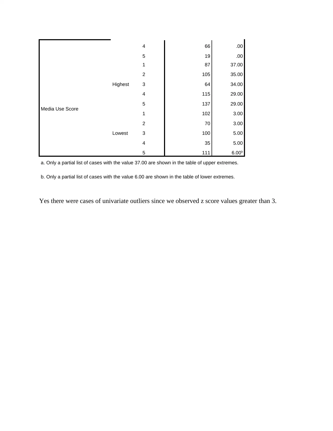
4 66 .00
5 19 .00
Media Use Score
Highest
1 87 37.00
2 105 35.00
3 64 34.00
4 115 29.00
5 137 29.00
Lowest
1 102 3.00
2 70 3.00
3 100 5.00
4 35 5.00
5 111 6.00b
a. Only a partial list of cases with the value 37.00 are shown in the table of upper extremes.
b. Only a partial list of cases with the value 6.00 are shown in the table of lower extremes.
Yes there were cases of univariate outliers since we observed z score values greater than 3.

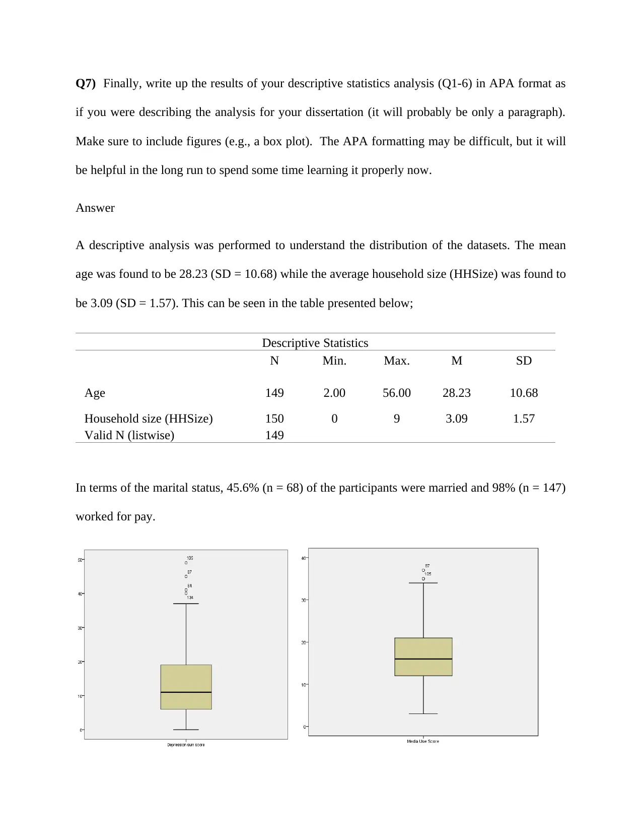
Q7) Finally, write up the results of your descriptive statistics analysis (Q1-6) in APA format as
if you were describing the analysis for your dissertation (it will probably be only a paragraph).
Make sure to include figures (e.g., a box plot). The APA formatting may be difficult, but it will
be helpful in the long run to spend some time learning it properly now.
Answer
A descriptive analysis was performed to understand the distribution of the datasets. The mean
age was found to be 28.23 (SD = 10.68) while the average household size (HHSize) was found to
be 3.09 (SD = 1.57). This can be seen in the table presented below;
Descriptive Statistics
N Min. Max. M SD
Age 149 2.00 56.00 28.23 10.68
Household size (HHSize) 150 0 9 3.09 1.57
Valid N (listwise) 149
In terms of the marital status, 45.6% (n = 68) of the participants were married and 98% (n = 147)
worked for pay.

From the boxplots constructed, the plots revealed that outliers were present in the Media use
score as well as the depression sum scores
There was however no pattern for the missing data but rather the data seemed to be missing at
random. The missing data were random for the various variables and not associated with say a
particular subject or particular item.
Part 2

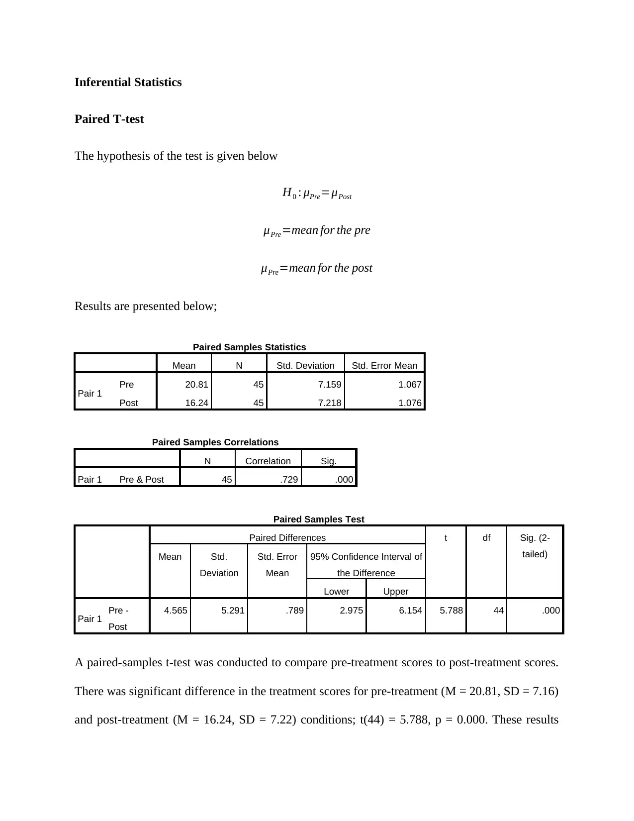
Inferential Statistics
Paired T-test
The hypothesis of the test is given below
H0 : μPre=μPost
μPre=mean for the pre
μPre=mean for the post
Results are presented below;
Paired Samples Statistics
Mean N Std. Deviation Std. Error Mean
Pair 1 Pre 20.81 45 7.159 1.067
Post 16.24 45 7.218 1.076
Paired Samples Correlations
N Correlation Sig.
Pair 1 Pre & Post 45 .729 .000
Paired Samples Test
Paired Differences t df Sig. (2-
tailed)Mean Std.
Deviation
Std. Error
Mean
95% Confidence Interval of
the Difference
Lower Upper
Pair 1 Pre -
Post
4.565 5.291 .789 2.975 6.154 5.788 44 .000
A paired-samples t-test was conducted to compare pre-treatment scores to post-treatment scores.
There was significant difference in the treatment scores for pre-treatment (M = 20.81, SD = 7.16)
and post-treatment (M = 16.24, SD = 7.22) conditions; t(44) = 5.788, p = 0.000. These results

suggest that there is a significant overall change between pre and post PTSD symptoms. The
overall treatment effect was quite significant in the sense that people get better over time.
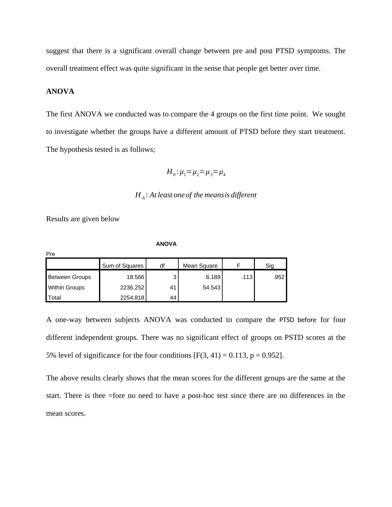
ANOVA
The first ANOVA we conducted was to compare the 4 groups on the first time point. We sought
to investigate whether the groups have a different amount of PTSD before they start treatment.
The hypothesis tested is as follows;
H0 : μ1=μ2=μ3=μ4
H A : At least one of the meansis different
Results are given below
ANOVA
Pre
Sum of Squares df Mean Square F Sig.
Between Groups 18.566 3 6.189 .113 .952
Within Groups 2236.252 41 54.543
Total 2254.818 44
A one-way between subjects ANOVA was conducted to compare the PTSD before for four
different independent groups. There was no significant effect of groups on PSTD scores at the
5% level of significance for the four conditions [F(3, 41) = 0.113, p = 0.952].
The above results clearly shows that the mean scores for the different groups are the same at the
start. There is thee =fore no need to have a post-hoc test since there are no differences in the
mean scores.

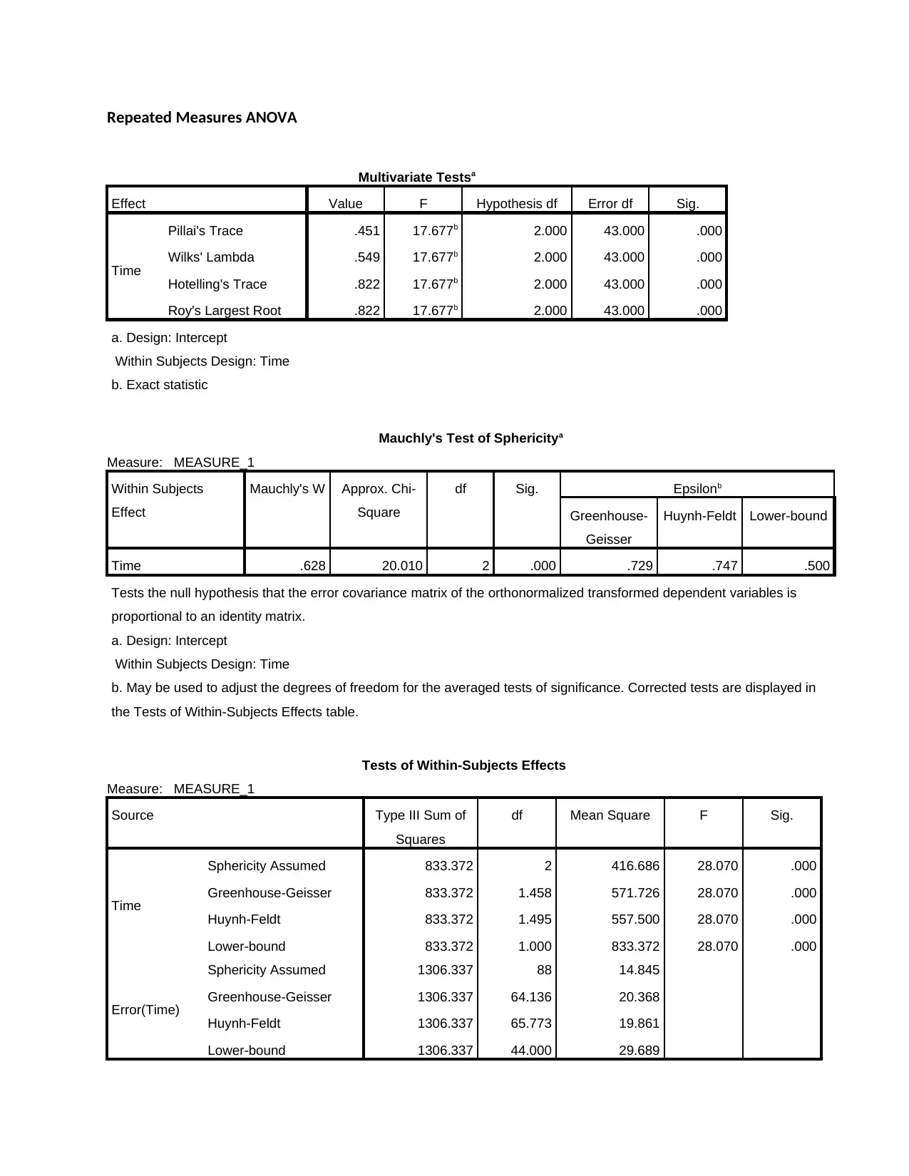
Repeated Measures ANOVA
Multivariate Testsa
Effect Value F Hypothesis df Error df Sig.
Time
Pillai's Trace .451 17.677b 2.000 43.000 .000
Wilks' Lambda .549 17.677b 2.000 43.000 .000
Hotelling's Trace .822 17.677b 2.000 43.000 .000
Roy's Largest Root .822 17.677b 2.000 43.000 .000
a. Design: Intercept
Within Subjects Design: Time
b. Exact statistic
Mauchly's Test of Sphericitya
Measure: MEASURE_1
Within Subjects
Effect
Mauchly's W Approx. Chi-
Square
df Sig. Epsilonb
Greenhouse-
Geisser
Huynh-Feldt Lower-bound
Time .628 20.010 2 .000 .729 .747 .500
Tests the null hypothesis that the error covariance matrix of the orthonormalized transformed dependent variables is
proportional to an identity matrix.
a. Design: Intercept
Within Subjects Design: Time
b. May be used to adjust the degrees of freedom for the averaged tests of significance. Corrected tests are displayed in
the Tests of Within-Subjects Effects table.
Tests of Within-Subjects Effects
Measure: MEASURE_1
Source Type III Sum of
Squares
df Mean Square F Sig.
Time
Sphericity Assumed 833.372 2 416.686 28.070 .000
Greenhouse-Geisser 833.372 1.458 571.726 28.070 .000
Huynh-Feldt 833.372 1.495 557.500 28.070 .000
Lower-bound 833.372 1.000 833.372 28.070 .000
Error(Time)
Sphericity Assumed 1306.337 88 14.845
Greenhouse-Geisser 1306.337 64.136 20.368
Huynh-Feldt 1306.337 65.773 19.861
Lower-bound 1306.337 44.000 29.689

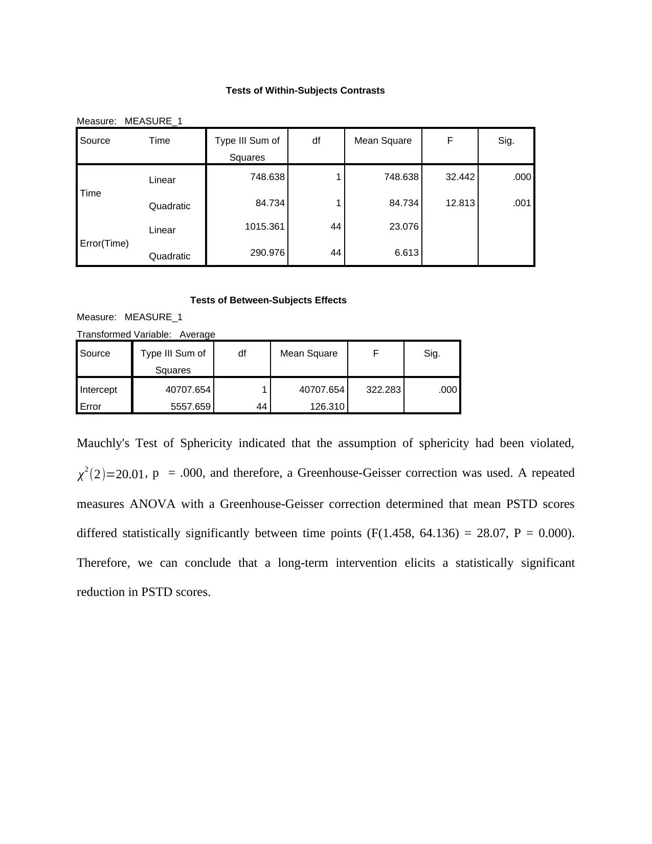
Tests of Within-Subjects Contrasts
Measure: MEASURE_1
Source Time Type III Sum of
Squares
df Mean Square F Sig.
Time
Linear 748.638 1 748.638 32.442 .000
Quadratic 84.734 1 84.734 12.813 .001
Error(Time)
Linear 1015.361 44 23.076
Quadratic 290.976 44 6.613
Tests of Between-Subjects Effects
Measure: MEASURE_1
Transformed Variable: Average
Source Type III Sum of
Squares
df Mean Square F Sig.
Intercept 40707.654 1 40707.654 322.283 .000
Error 5557.659 44 126.310
Mauchly's Test of Sphericity indicated that the assumption of sphericity had been violated,
χ2 (2)=20.01, p = .000, and therefore, a Greenhouse-Geisser correction was used. A repeated
measures ANOVA with a Greenhouse-Geisser correction determined that mean PSTD scores
differed statistically significantly between time points (F(1.458, 64.136) = 28.07, P = 0.000).
Therefore, we can conclude that a long-term intervention elicits a statistically significant
reduction in PSTD scores.