Statistics for Management: Earnings and Regional Analysis Report

This report presents a statistical analysis of earnings data, focusing on comparisons between men and women in the public and private sectors. It utilizes hypothesis testing, specifically t-tests, to determine significant differences in earnings. The report includes time charts illustrating earnings trends over several years and calculates annual growth rates for different groups. Furthermore, the analysis extends to hourly pay rates across various UK regions, employing median calculations, quartile analysis, and standard deviation to assess pay disparities. Data visualization techniques, such as bar and pie charts, are used to present the findings and provide a clear understanding of the relationships between variables, such as the number of bedrooms and house prices in different streets. The report concludes by summarizing the key findings and their implications.

Statistics for Management

Table of Contents
INTRODUCTION...........................................................................................................................2
MAIN BODY...................................................................................................................................2
TASK 1............................................................................................................................................2
A. Determine how earnings of men in public sector is different from earnings of women in
public sector by using hypothesis................................................................................................2
B. Determine how earnings of men in private sector is different from earnings of women in
private sector by using hypothesis...............................................................................................3
C. Earning time chart of each group............................................................................................4
D. Evaluating the annual growth rate in the context of earnings of given four group.................6
TASK 2............................................................................................................................................8
A) Analysis and evaluation of hourly pay rates in different UK regions....................................8
B) Earnings comparison in between two regions......................................................................12
TASK 3 .........................................................................................................................................12
Section A....................................................................................................................................12
Section B....................................................................................................................................13
TASK 4 .........................................................................................................................................13
4.1...............................................................................................................................................13
1. Bar chart.................................................................................................................................13
2. Pie chart.................................................................................................................................16
....................................................................................................................................................18
4.2 Relationship between the number of bedrooms and the house price of bedrooms in all of
the three streets..........................................................................................................................19
CONCLUSION..............................................................................................................................25
REFERENCES..............................................................................................................................26
1

INTRODUCTION
Statistics is a term which is related with the process of data collection, analysis as well as
interpretation so as to ascertain some meaningful information from it. With the help of
mathematical as well as statistical tools, data gathered can be evaluated in effective manner.
Also, by making use of different types of graphs, charts presentation of numerical data provides
better understanding to end users and assists in their decision making process. The present report
will define about economic data with the help of time chart. Furthermore, with the help of
comparison among hourly earnings of two different regions, statistical meaning will be derive.
Also, by applying statistical methods such as Economic order quantity, normal distribution
curves etc. explanation related to different section will be done. At last, the report will made
emphasis on making presentation of given data set in both the bar as well as pie chart form.
MAIN BODY
TASK 1
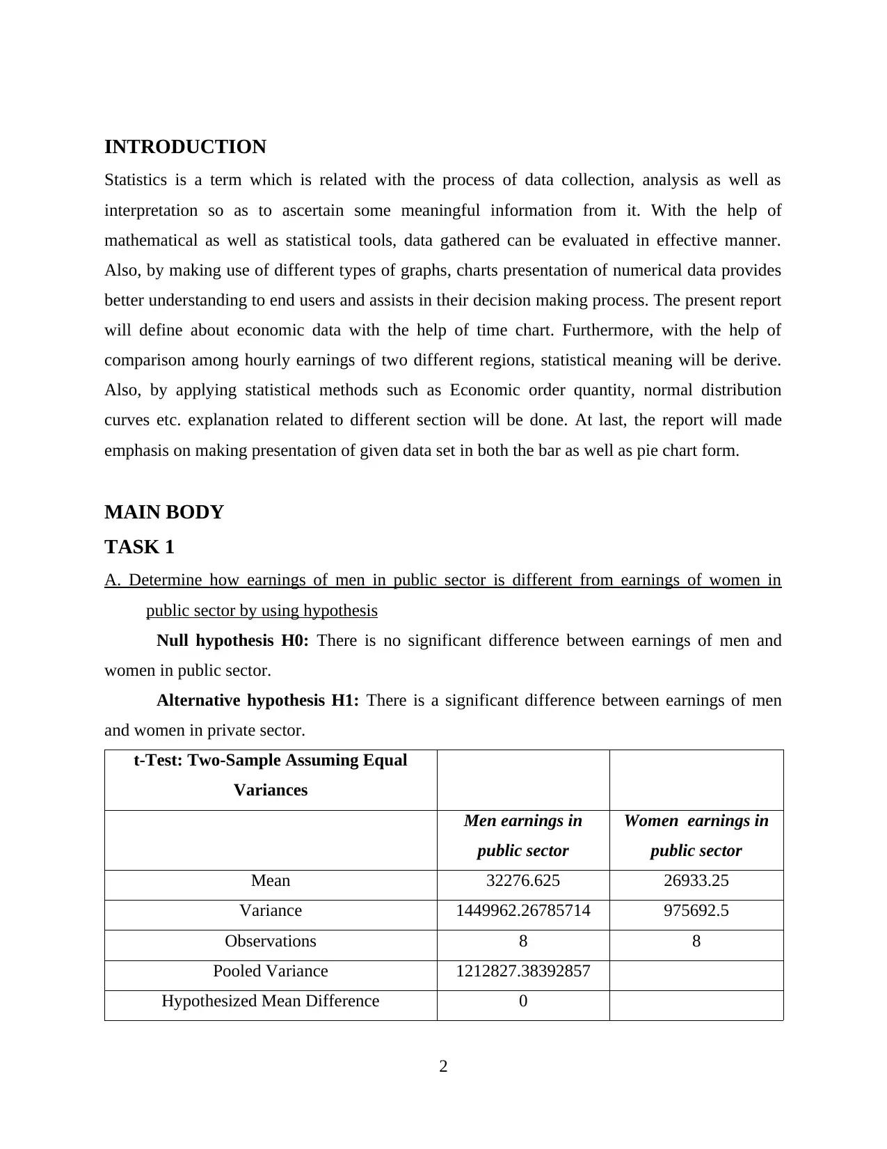
A. Determine how earnings of men in public sector is different from earnings of women in
public sector by using hypothesis
Null hypothesis H0: There is no significant difference between earnings of men and
women in public sector.
Alternative hypothesis H1: There is a significant difference between earnings of men
and women in private sector.
t-Test: Two-Sample Assuming Equal
Variances
Men earnings in
public sector
Women earnings in
public sector
Mean 32276.625 26933.25
Variance 1449962.26785714 975692.5
Observations 8 8
Pooled Variance 1212827.38392857
Hypothesized Mean Difference 0
2

df 14
t Stat 9.7038964331
P(T<=t) one-tail
6.76878422104249E-
008
t Critical one-tail 1.7613101358
P(T<=t) two-tail 1.3537568442085E-007
t Critical two-tail 2.1447866879
Interpretation - From the above table it can be interpreted that null hypothesis will be
accepted as 1.35 is greater than 0.05 depicting about no significant difference in between the
earnings of men and women working in the public sector. No discrimination has been made on
gender basis in the context of income payment. Equal pay and status has been provided to both
the genders as per the Government norms and regulations as well (Berman and Wang, 2016).
Thus it can be said that because of no significant difference among earnings of men and women
working in the public sector, it has assisted in improving standard of living.
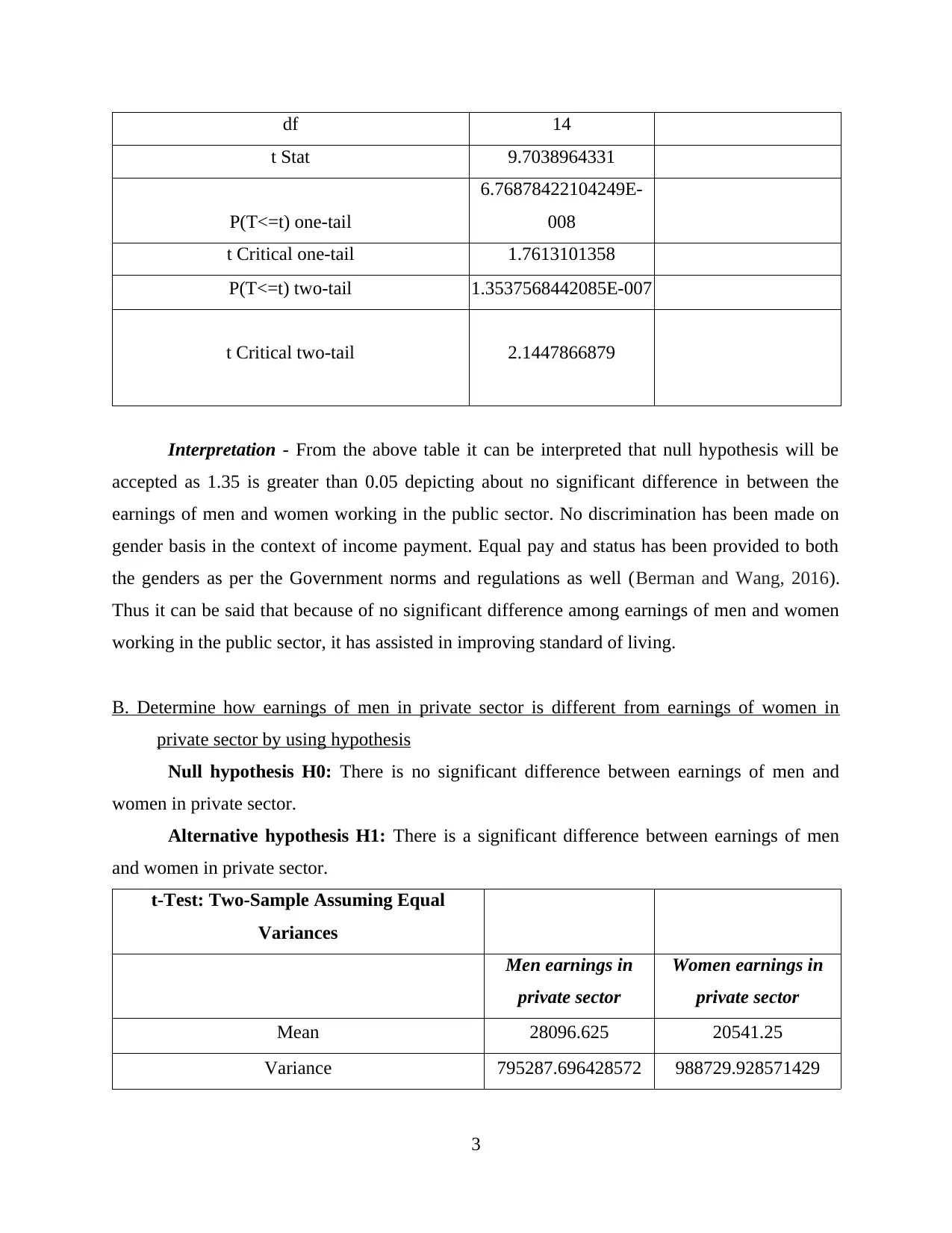
B. Determine how earnings of men in private sector is different from earnings of women in
private sector by using hypothesis
Null hypothesis H0: There is no significant difference between earnings of men and
women in private sector.
Alternative hypothesis H1: There is a significant difference between earnings of men
and women in private sector.
t-Test: Two-Sample Assuming Equal
Variances
Men earnings in
private sector
Women earnings in
private sector
Mean 28096.625 20541.25
Variance 795287.696428572 988729.928571429
3

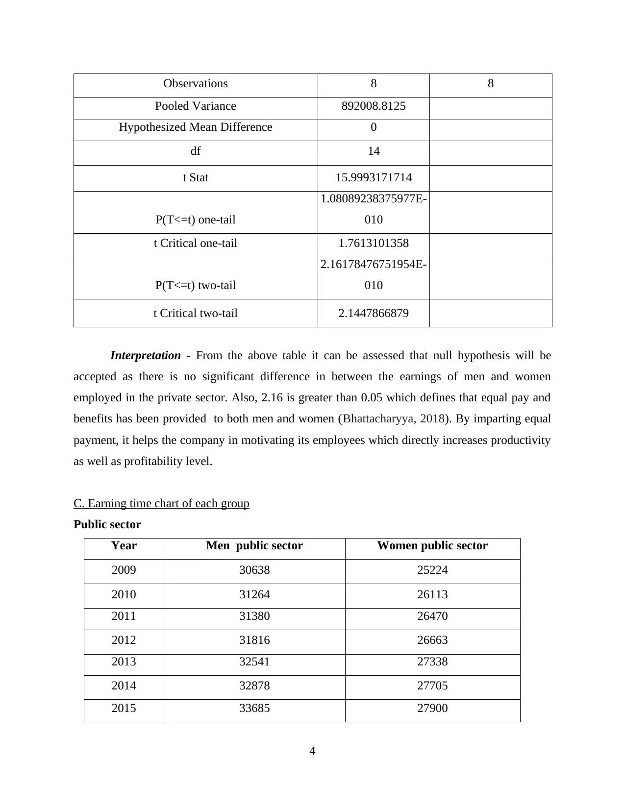
Observations 8 8
Pooled Variance 892008.8125
Hypothesized Mean Difference 0
df 14
t Stat 15.9993171714
P(T<=t) one-tail
1.08089238375977E-
010
t Critical one-tail 1.7613101358
P(T<=t) two-tail
2.16178476751954E-
010
t Critical two-tail 2.1447866879
Interpretation - From the above table it can be assessed that null hypothesis will be
accepted as there is no significant difference in between the earnings of men and women
employed in the private sector. Also, 2.16 is greater than 0.05 which defines that equal pay and
benefits has been provided to both men and women (Bhattacharyya, 2018). By imparting equal
payment, it helps the company in motivating its employees which directly increases productivity
as well as profitability level.
C. Earning time chart of each group
Public sector
Year Men public sector Women public sector
2009 30638 25224
2010 31264 26113
2011 31380 26470
2012 31816 26663
2013 32541 27338
2014 32878 27705
2015 33685 27900
4

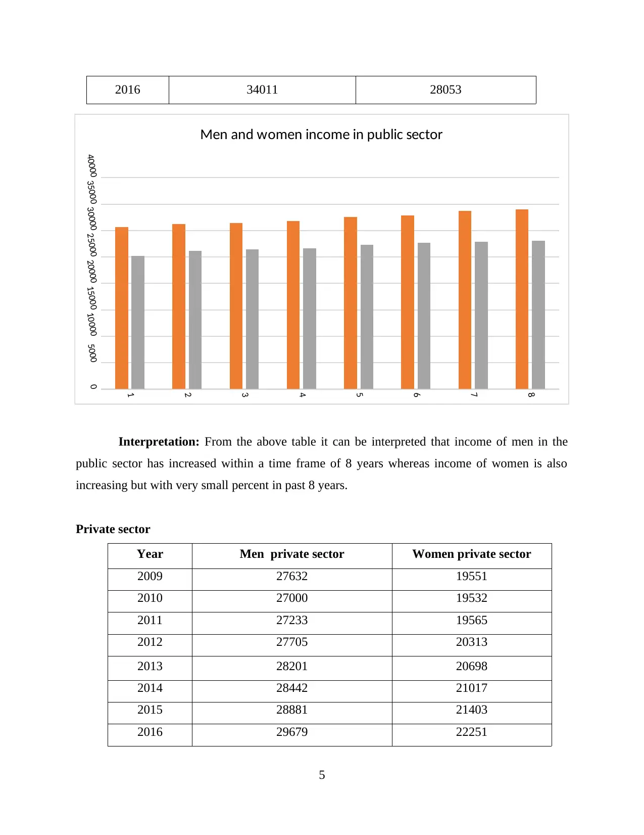
2016 34011 28053
Interpretation: From the above table it can be interpreted that income of men in the
public sector has increased within a time frame of 8 years whereas income of women is also
increasing but with very small percent in past 8 years.
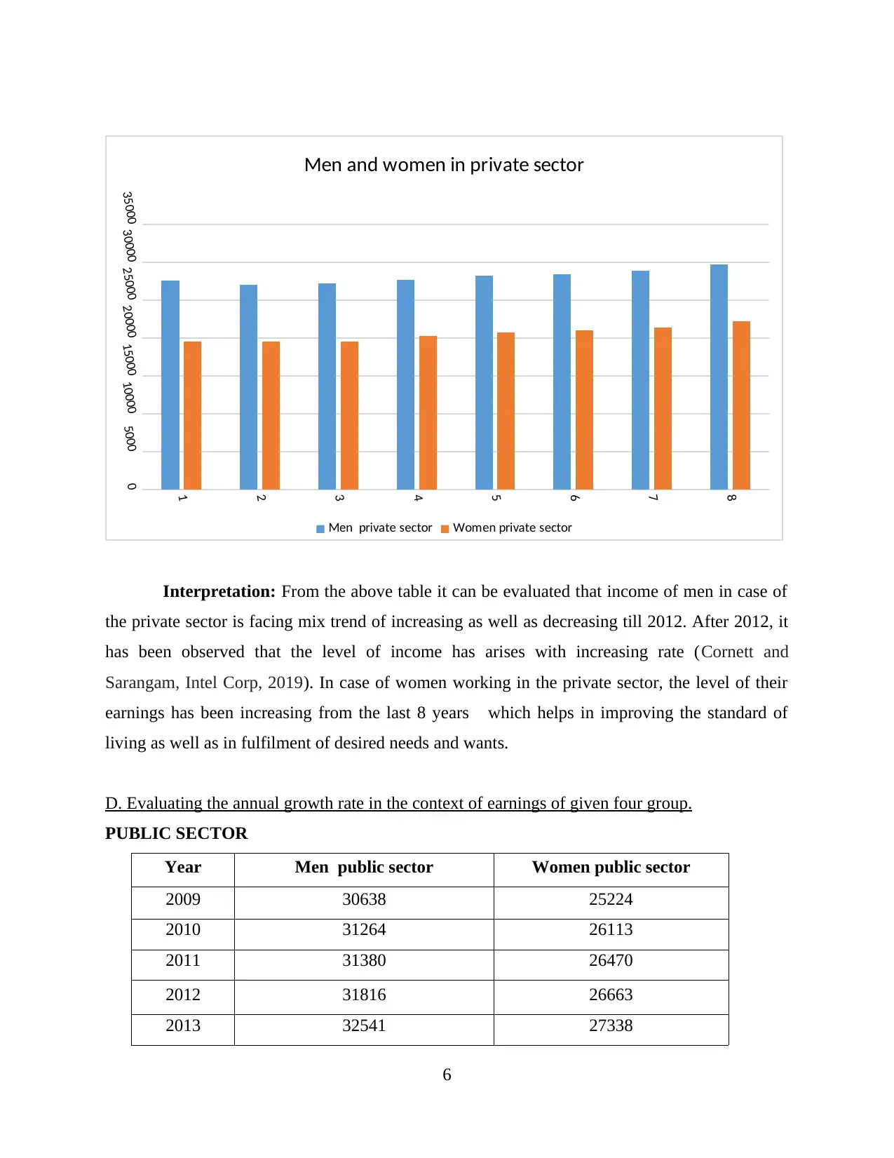
Private sector
Year Men private sector Women private sector
2009 27632 19551
2010 27000 19532
2011 27233 19565
2012 27705 20313
2013 28201 20698
2014 28442 21017
2015 28881 21403
2016 29679 22251
5
1
2
3
4
5
6
7
8
0500010000150002000025000300003500040000
Men and women income in public sector

1
2
3
4
5
6
7
8
0
5000
10000
15000
20000
25000
30000
35000
Men and women in private sector
Men private sector Women private sector
Interpretation: From the above table it can be evaluated that income of men in case of
the private sector is facing mix trend of increasing as well as decreasing till 2012. After 2012, it
has been observed that the level of income has arises with increasing rate (Cornett and
Sarangam, Intel Corp, 2019). In case of women working in the private sector, the level of their
earnings has been increasing from the last 8 years which helps in improving the standard of
living as well as in fulfilment of desired needs and wants.
D. Evaluating the annual growth rate in the context of earnings of given four group.
PUBLIC SECTOR
Year Men public sector Women public sector
2009 30638 25224
2010 31264 26113
2011 31380 26470
2012 31816 26663
2013 32541 27338
6

2014 32878 27705
2015 33685 27900
2016 34011 28053
ANNUAL GROWTH RATE
Year Men public
sector
YOY Growth
rate
Women public
sector
YOY Growth
rate
2009 30638 25224
2010 31264 2% 26113 4%
2011 31380 0% 26470 1%
2012 31816 1% 26663 1%
2013 32541 2% 27338 3%
2014 32878 1% 27705 1%
2015 33685 2% 27900 1%
2016 34011 1% 28053 1%
Interpretation – As per the given table, it can be assessed that the YOY growth rate of
Men is showing declining trend when compared among year 2015 to the year 2016. The growth
rate of earnings of men as employed in the public sector has declined from 2% in 2010 to 1% in
the year 2016 (De Vries and Hitomi, Numecent Holdings Inc, 2016). On the other hand, the
YOY annual growth rate of women was 4% in the year 2010 which has declined to 1% in the
year 2011. It signifies that the financial progress of women working in the public sector firms are
not showing positive returns.
PRIVATE SECTOR
Year Men private sector Women private sector
2009 27632 19551
2010 27000 19532
2011 27233 19565
2012 27705 20313
7

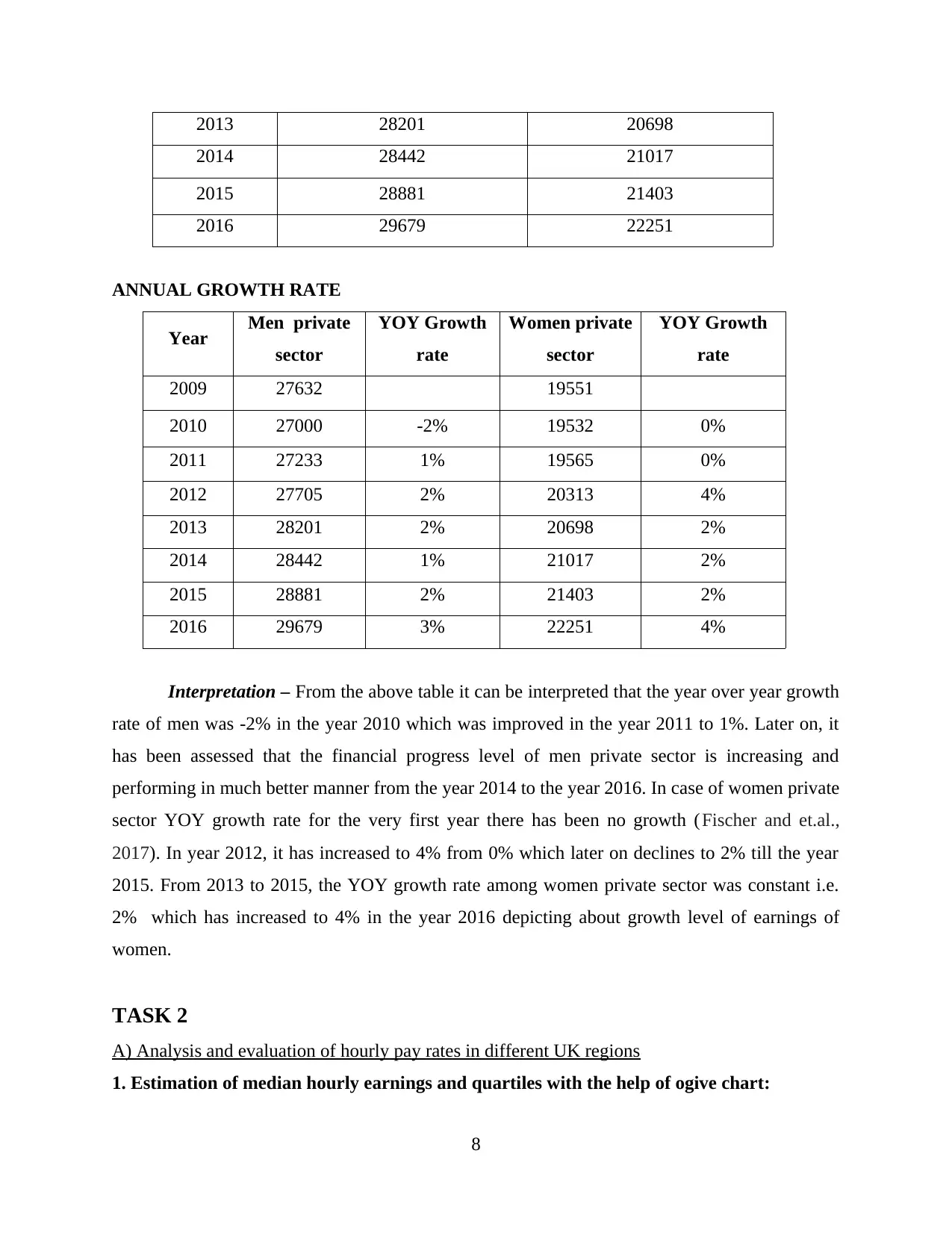
2013 28201 20698
2014 28442 21017
2015 28881 21403
2016 29679 22251
ANNUAL GROWTH RATE
Year Men private
sector
YOY Growth
rate
Women private
sector
YOY Growth
rate
2009 27632 19551
2010 27000 -2% 19532 0%
2011 27233 1% 19565 0%
2012 27705 2% 20313 4%
2013 28201 2% 20698 2%
2014 28442 1% 21017 2%
2015 28881 2% 21403 2%
2016 29679 3% 22251 4%
Interpretation – From the above table it can be interpreted that the year over year growth
rate of men was -2% in the year 2010 which was improved in the year 2011 to 1%. Later on, it
has been assessed that the financial progress level of men private sector is increasing and
performing in much better manner from the year 2014 to the year 2016. In case of women private
sector YOY growth rate for the very first year there has been no growth (Fischer and et.al.,
2017). In year 2012, it has increased to 4% from 0% which later on declines to 2% till the year
2015. From 2013 to 2015, the YOY growth rate among women private sector was constant i.e.
2% which has increased to 4% in the year 2016 depicting about growth level of earnings of
women.
TASK 2
A) Analysis and evaluation of hourly pay rates in different UK regions
1. Estimation of median hourly earnings and quartiles with the help of ogive chart:
8

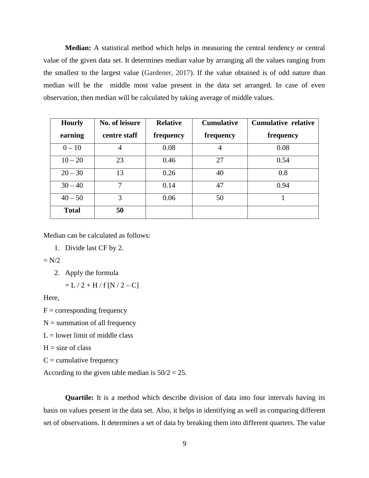
Median: A statistical method which helps in measuring the central tendency or central
value of the given data set. It determines median value by arranging all the values ranging from
the smallest to the largest value (Gardener, 2017). If the value obtained is of odd nature than
median will be the middle most value present in the data set arranged. In case of even
observation, then median will be calculated by taking average of middle values.
Hourly
earning
No. of leisure
centre staff
Relative
frequency
Cumulative
frequency
Cumulative relative
frequency
0 – 10 4 0.08 4 0.08
10 – 20 23 0.46 27 0.54
20 – 30 13 0.26 40 0.8
30 – 40 7 0.14 47 0.94
40 – 50 3 0.06 50 1
Total 50
Median can be calculated as follows:
1. Divide last CF by 2.
= N/2
2. Apply the formula
= L / 2 + H / f [N / 2 – C]
Here,
F = corresponding frequency
N = summation of all frequency
L = lower limit of middle class
H = size of class
C = cumulative frequency
According to the given table median is 50/2 = 25.
Quartile: It is a method which describe division of data into four intervals having its
basis on values present in the data set. Also, it helps in identifying as well as comparing different
set of observations. It determines a set of data by breaking them into different quarters. The value
9

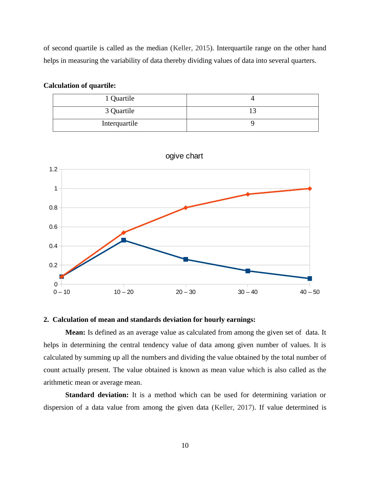
of second quartile is called as the median (Keller, 2015). Interquartile range on the other hand
helps in measuring the variability of data thereby dividing values of data into several quarters.
Calculation of quartile:
1 Quartile 4
3 Quartile 13
Interquartile 9
0 – 10 10 – 20 20 – 30 30 – 40 40 – 50
0
0.2
0.4
0.6
0.8
1
1.2
ogive chart
2. Calculation of mean and standards deviation for hourly earnings:
Mean: Is defined as an average value as calculated from among the given set of data. It
helps in determining the central tendency value of data among given number of values. It is
calculated by summing up all the numbers and dividing the value obtained by the total number of
count actually present. The value obtained is known as mean value which is also called as the
arithmetic mean or average mean.
Standard deviation: It is a method which can be used for determining variation or
dispersion of a data value from among the given data (Keller, 2017). If value determined is
10

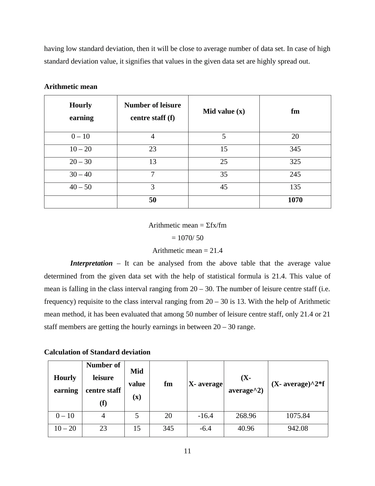
having low standard deviation, then it will be close to average number of data set. In case of high
standard deviation value, it signifies that values in the given data set are highly spread out.
Arithmetic mean
Hourly
earning
Number of leisure
centre staff (f) Mid value (x) fm
0 – 10 4 5 20
10 – 20 23 15 345
20 – 30 13 25 325
30 – 40 7 35 245
40 – 50 3 45 135
50 1070
Arithmetic mean = Σfx/fm
= 1070/ 50
Arithmetic mean = 21.4
Interpretation – It can be analysed from the above table that the average value
determined from the given data set with the help of statistical formula is 21.4. This value of
mean is falling in the class interval ranging from 20 – 30. The number of leisure centre staff (i.e.
frequency) requisite to the class interval ranging from 20 – 30 is 13. With the help of Arithmetic
mean method, it has been evaluated that among 50 number of leisure centre staff, only 21.4 or 21
staff members are getting the hourly earnings in between 20 – 30 range.
Calculation of Standard deviation
Hourly
earning
Number of
leisure
centre staff
(f)
Mid
value
(x)
fm X- average (X-
average^2) (X- average)^2*f
0 – 10 4 5 20 -16.4 268.96 1075.84
10 – 20 23 15 345 -6.4 40.96 942.08
11