Statistics for Management: Report on Earnings and Salary Statistics
VerifiedAdded on 2020/10/22
|15
|3020
|285
Report
AI Summary
This report presents a statistical analysis of gross annual earnings in both public and private sectors from 2010 to 2016, examining trends and changes in male and female salaries. The analysis includes calculations of percentage changes, comparisons of gender pay gaps, and an examination of earnings differences between education and finance sectors. Further, the report calculates mean and standard deviation for hourly earnings, utilizes ogive charts to estimate median hourly earnings and quartiles, and compares earnings between two regions. The report also includes a hypothesis test to determine the independence of mobile phone choice and annual salary, and concludes with a line chart visualizing earnings trends over the years. The report uses statistical methods to interpret the data and draw conclusions about salary trends and disparities.

STATISTICS FOR
MANAGEMENT
MANAGEMENT
Paraphrase This Document
Need a fresh take? Get an instant paraphrase of this document with our AI Paraphraser
TABLE OF CONTENTS
INTRODUCTION...........................................................................................................................1
ACTIVITY 1 (LO 1)........................................................................................................................1
1. Calculating changes in gross annual earnings in public and private sectors...........................1
Gross annual earning in public sector (male)..............................................................................1
Gross annual earning in public sector (female)...........................................................................1
Gross annual earning in private sector (male).............................................................................2
Gross annual earnings in private sector (female) .......................................................................2
2. Analysing male and female gross annual earning among 2010 to 2016.................................2
3. Analysing the gap between education and finance gross annual earnings..............................3
4. Examining comparison for better earnings of staff in health and social care and to
administrative staff......................................................................................................................3
ACTIVITY 2....................................................................................................................................4
A.1 Using ogive for estimating the median hourly earnings and the quartiles...........................4
A.2 Calculating the mean and standard deviation for hourly earnings.......................................6
(b.) Comparing the earnings between the two regions................................................................7
ACTIVITY 3 (LO 3)- CLIENT C...................................................................................................7
1. Stating a suitable hypothesis for testing the claim..................................................................7
2. Using a statistical test, determining a mobile phone choice which is independent of annual
salary ..........................................................................................................................................8
ACTIVITY 4....................................................................................................................................9
1. Producing a line chart which indicating both male and female gross annual earnings for
public and private sectors form the year 2010 to 2016...............................................................9
Analysing gross annual earnings of female in both the sectors................................................10
CONCLUSION..............................................................................................................................11
REFERENCES..............................................................................................................................12

⊘ This is a preview!⊘
Do you want full access?
Subscribe today to unlock all pages.
Trusted by 1+ million students worldwide
INTRODUCTION
Statistics is a concept which considered as the branch of mathematics in order to deal
with data which collected for organisation, analysis, interpretation and for presentation. It is
highly interdisciplinary field which mainly used in the field of research (Keller, 2015). Thus, in
this report evaluation will be conducted on the gross annual earnings in both public and private
sector which has changes since 2010 with gap between the earnings of male and female. Further,
calculation will be provided on mean and standard deviation for hourly earnings and evaluation
will also be conducted on earning between the two regions.
ACTIVITY 1 (LO 1)
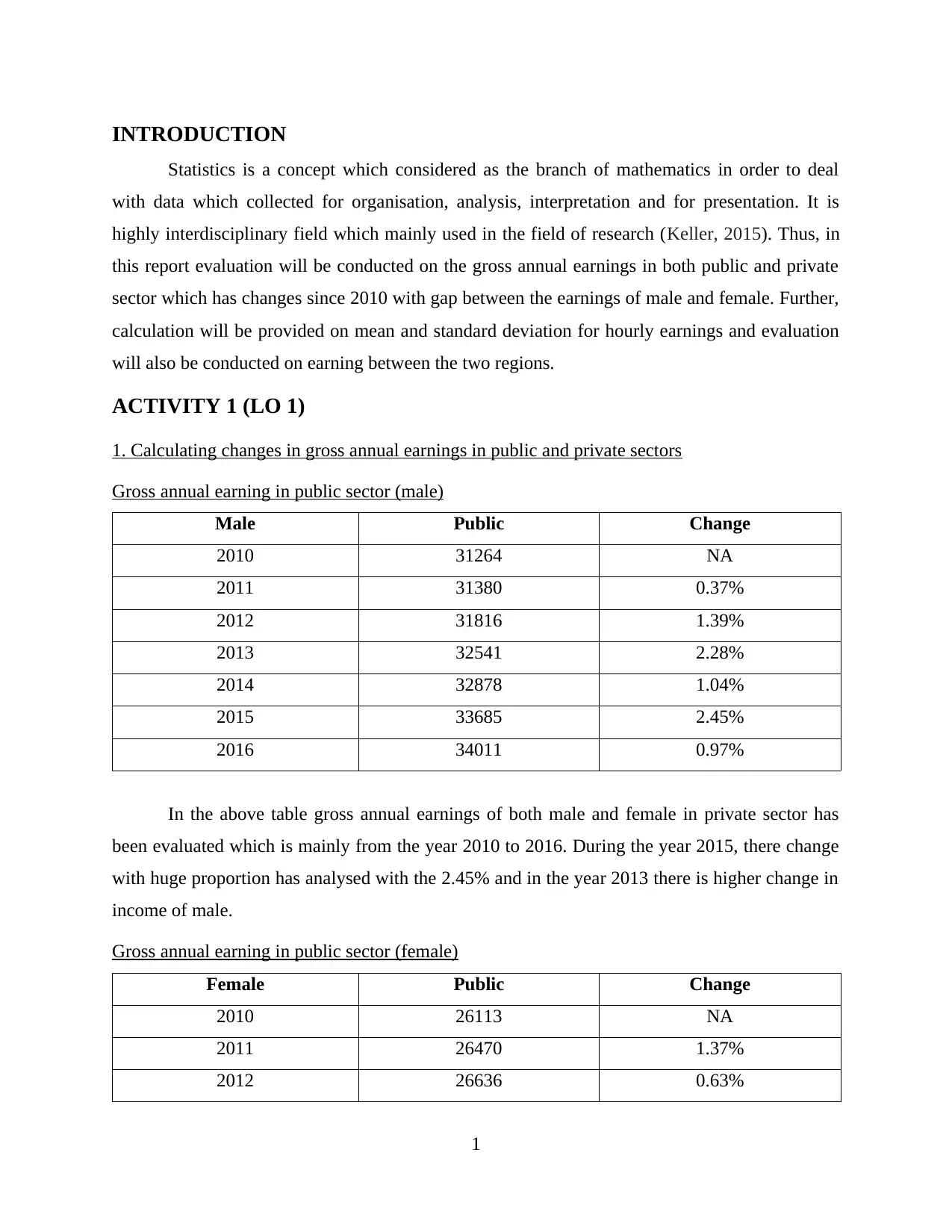
1. Calculating changes in gross annual earnings in public and private sectors
Gross annual earning in public sector (male)
Male Public Change
2010 31264 NA
2011 31380 0.37%
2012 31816 1.39%
2013 32541 2.28%
2014 32878 1.04%
2015 33685 2.45%
2016 34011 0.97%
In the above table gross annual earnings of both male and female in private sector has
been evaluated which is mainly from the year 2010 to 2016. During the year 2015, there change
with huge proportion has analysed with the 2.45% and in the year 2013 there is higher change in
income of male.
Gross annual earning in public sector (female)
Female Public Change
2010 26113 NA
2011 26470 1.37%
2012 26636 0.63%
1
Statistics is a concept which considered as the branch of mathematics in order to deal
with data which collected for organisation, analysis, interpretation and for presentation. It is
highly interdisciplinary field which mainly used in the field of research (Keller, 2015). Thus, in
this report evaluation will be conducted on the gross annual earnings in both public and private
sector which has changes since 2010 with gap between the earnings of male and female. Further,
calculation will be provided on mean and standard deviation for hourly earnings and evaluation
will also be conducted on earning between the two regions.
ACTIVITY 1 (LO 1)
1. Calculating changes in gross annual earnings in public and private sectors
Gross annual earning in public sector (male)
Male Public Change
2010 31264 NA
2011 31380 0.37%
2012 31816 1.39%
2013 32541 2.28%
2014 32878 1.04%
2015 33685 2.45%
2016 34011 0.97%
In the above table gross annual earnings of both male and female in private sector has
been evaluated which is mainly from the year 2010 to 2016. During the year 2015, there change
with huge proportion has analysed with the 2.45% and in the year 2013 there is higher change in
income of male.
Gross annual earning in public sector (female)
Female Public Change
2010 26113 NA
2011 26470 1.37%
2012 26636 0.63%
1
Paraphrase This Document
Need a fresh take? Get an instant paraphrase of this document with our AI Paraphraser
2013 27338 2.64%
2014 27705 1.34%
2015 27905 0.72%
2016 28053 0.53%
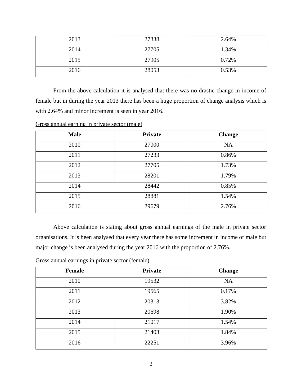
From the above calculation it is analysed that there was no drastic change in income of
female but in during the year 2013 there has been a huge proportion of change analysis which is
with 2.64% and minor increment is seen in year 2016.
Gross annual earning in private sector (male)
Male Private Change
2010 27000 NA
2011 27233 0.86%
2012 27705 1.73%
2013 28201 1.79%
2014 28442 0.85%
2015 28881 1.54%
2016 29679 2.76%
Above calculation is stating about gross annual earnings of the male in private sector
organisations. It is been analysed that every year there has some increment in income of male but
major change is been analysed during the year 2016 with the proportion of 2.76%.
Gross annual earnings in private sector (female)
Female Private Change
2010 19532 NA
2011 19565 0.17%
2012 20313 3.82%
2013 20698 1.90%
2014 21017 1.54%
2015 21403 1.84%
2016 22251 3.96%
2
2014 27705 1.34%
2015 27905 0.72%
2016 28053 0.53%
From the above calculation it is analysed that there was no drastic change in income of
female but in during the year 2013 there has been a huge proportion of change analysis which is
with 2.64% and minor increment is seen in year 2016.
Gross annual earning in private sector (male)
Male Private Change
2010 27000 NA
2011 27233 0.86%
2012 27705 1.73%
2013 28201 1.79%
2014 28442 0.85%
2015 28881 1.54%
2016 29679 2.76%
Above calculation is stating about gross annual earnings of the male in private sector
organisations. It is been analysed that every year there has some increment in income of male but
major change is been analysed during the year 2016 with the proportion of 2.76%.
Gross annual earnings in private sector (female)
Female Private Change
2010 19532 NA
2011 19565 0.17%
2012 20313 3.82%
2013 20698 1.90%
2014 21017 1.54%
2015 21403 1.84%
2016 22251 3.96%
2
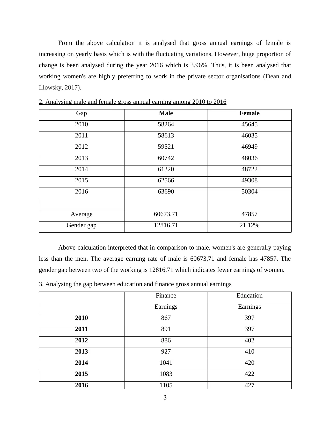
From the above calculation it is analysed that gross annual earnings of female is
increasing on yearly basis which is with the fluctuating variations. However, huge proportion of
change is been analysed during the year 2016 which is 3.96%. Thus, it is been analysed that
working women's are highly preferring to work in the private sector organisations (Dean and
Illowsky, 2017).
2. Analysing male and female gross annual earning among 2010 to 2016
Gap Male Female
2010 58264 45645
2011 58613 46035
2012 59521 46949
2013 60742 48036
2014 61320 48722
2015 62566 49308
2016 63690 50304
Average 60673.71 47857
Gender gap 12816.71 21.12%
Above calculation interpreted that in comparison to male, women's are generally paying
less than the men. The average earning rate of male is 60673.71 and female has 47857. The
gender gap between two of the working is 12816.71 which indicates fewer earnings of women.
3. Analysing the gap between education and finance gross annual earnings
Finance Education
Earnings Earnings
2010 867 397
2011 891 397
2012 886 402
2013 927 410
2014 1041 420
2015 1083 422
2016 1105 427
3
⊘ This is a preview!⊘
Do you want full access?
Subscribe today to unlock all pages.
Trusted by 1+ million students worldwide
2017 1194 440
2018 1210 454
Average 1023 419
Gap 604 59%
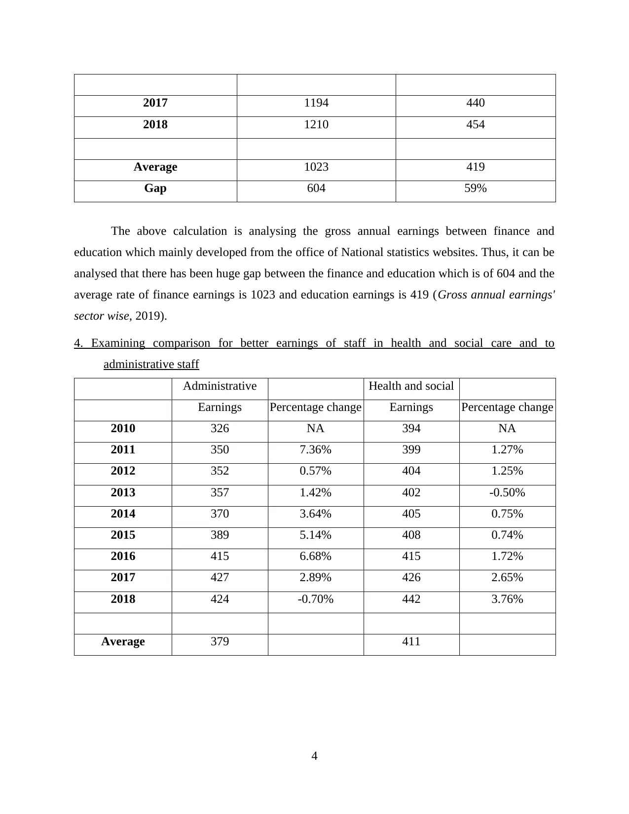
The above calculation is analysing the gross annual earnings between finance and
education which mainly developed from the office of National statistics websites. Thus, it can be
analysed that there has been huge gap between the finance and education which is of 604 and the
average rate of finance earnings is 1023 and education earnings is 419 (Gross annual earnings'
sector wise, 2019).
4. Examining comparison for better earnings of staff in health and social care and to
administrative staff
Administrative Health and social
Earnings Percentage change Earnings Percentage change
2010 326 NA 394 NA
2011 350 7.36% 399 1.27%
2012 352 0.57% 404 1.25%
2013 357 1.42% 402 -0.50%
2014 370 3.64% 405 0.75%
2015 389 5.14% 408 0.74%
2016 415 6.68% 415 1.72%
2017 427 2.89% 426 2.65%
2018 424 -0.70% 442 3.76%
Average 379 411
4
2018 1210 454
Average 1023 419
Gap 604 59%
The above calculation is analysing the gross annual earnings between finance and
education which mainly developed from the office of National statistics websites. Thus, it can be
analysed that there has been huge gap between the finance and education which is of 604 and the
average rate of finance earnings is 1023 and education earnings is 419 (Gross annual earnings'
sector wise, 2019).
4. Examining comparison for better earnings of staff in health and social care and to
administrative staff
Administrative Health and social
Earnings Percentage change Earnings Percentage change
2010 326 NA 394 NA
2011 350 7.36% 399 1.27%
2012 352 0.57% 404 1.25%
2013 357 1.42% 402 -0.50%
2014 370 3.64% 405 0.75%
2015 389 5.14% 408 0.74%
2016 415 6.68% 415 1.72%
2017 427 2.89% 426 2.65%
2018 424 -0.70% 442 3.76%
Average 379 411
4
Paraphrase This Document
Need a fresh take? Get an instant paraphrase of this document with our AI Paraphraser
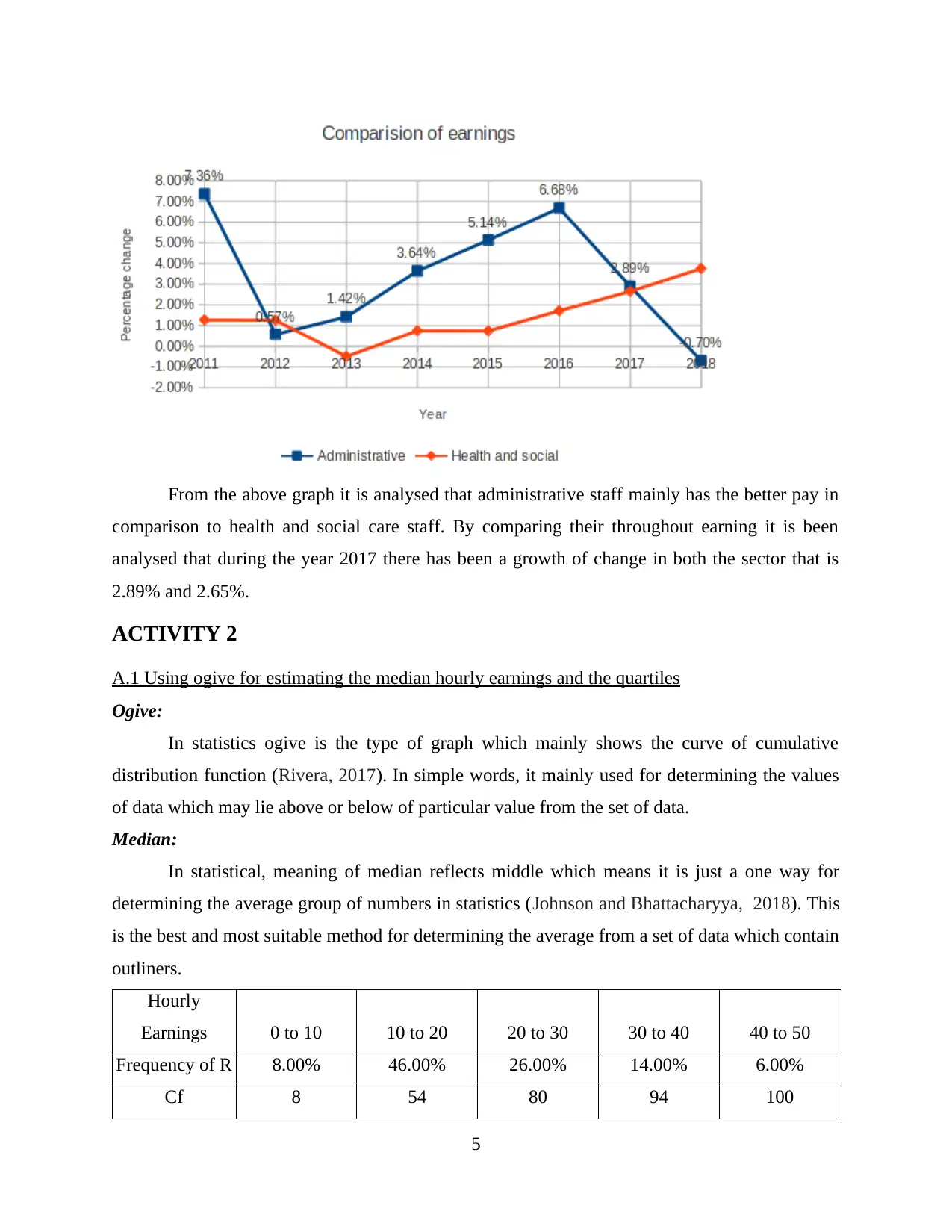
From the above graph it is analysed that administrative staff mainly has the better pay in
comparison to health and social care staff. By comparing their throughout earning it is been
analysed that during the year 2017 there has been a growth of change in both the sector that is
2.89% and 2.65%.
ACTIVITY 2
A.1 Using ogive for estimating the median hourly earnings and the quartiles
Ogive:
In statistics ogive is the type of graph which mainly shows the curve of cumulative
distribution function (Rivera, 2017). In simple words, it mainly used for determining the values
of data which may lie above or below of particular value from the set of data.
Median:
In statistical, meaning of median reflects middle which means it is just a one way for
determining the average group of numbers in statistics (Johnson and Bhattacharyya, 2018). This
is the best and most suitable method for determining the average from a set of data which contain
outliners.
Hourly
Earnings 0 to 10 10 to 20 20 to 30 30 to 40 40 to 50
Frequency of R 8.00% 46.00% 26.00% 14.00% 6.00%
Cf 8 54 80 94 100
5
CRF 8.00% 54.00% 80.00% 94.00% 100.00%
Hourly Earnings Employees (F) Cf
0 to 10 8 8
10 to 20 46 54
20 to 30 26 80
30 to 40 14 94
40 to 50 6 100
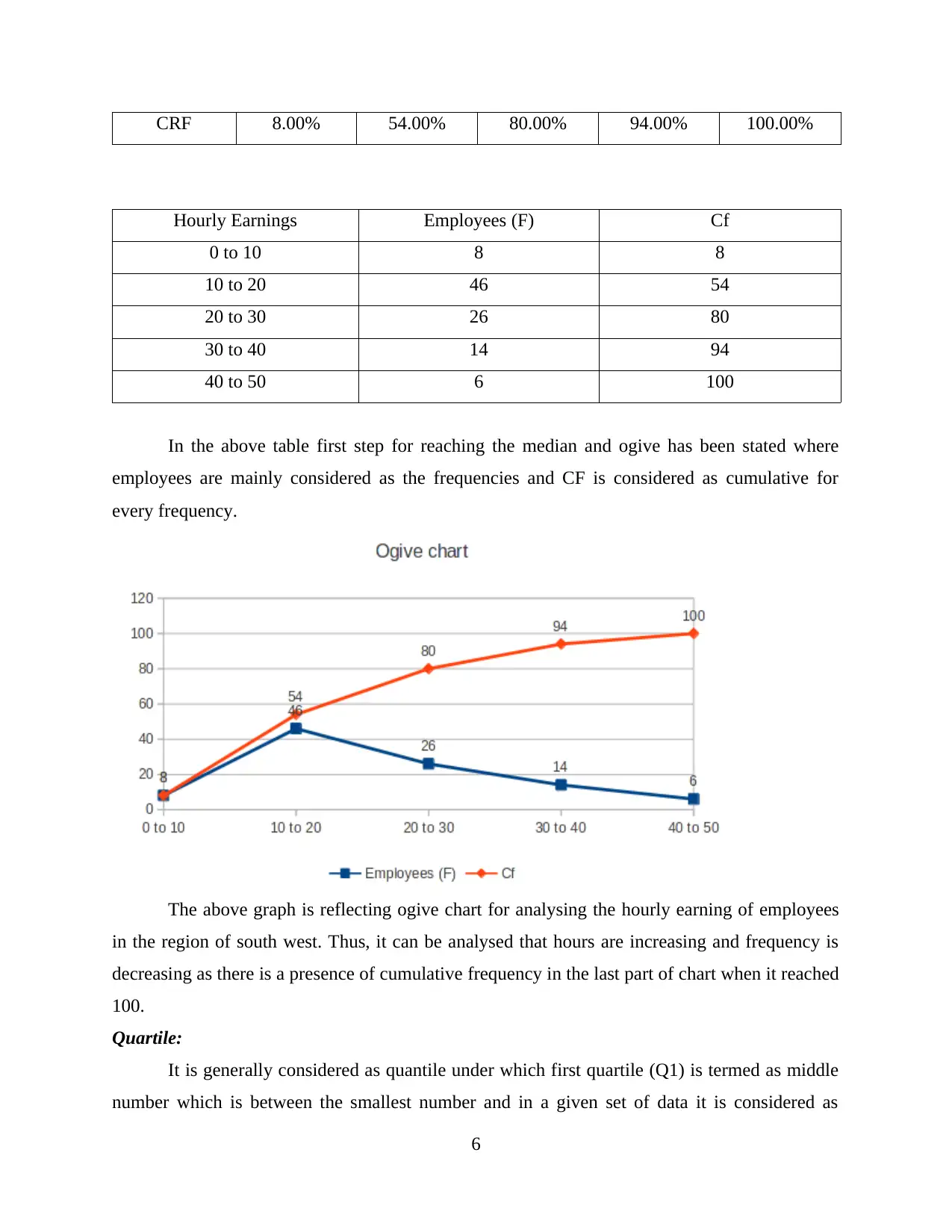
In the above table first step for reaching the median and ogive has been stated where
employees are mainly considered as the frequencies and CF is considered as cumulative for
every frequency.
The above graph is reflecting ogive chart for analysing the hourly earning of employees
in the region of south west. Thus, it can be analysed that hours are increasing and frequency is
decreasing as there is a presence of cumulative frequency in the last part of chart when it reached
100.
Quartile:
It is generally considered as quantile under which first quartile (Q1) is termed as middle
number which is between the smallest number and in a given set of data it is considered as
6
Hourly Earnings Employees (F) Cf
0 to 10 8 8
10 to 20 46 54
20 to 30 26 80
30 to 40 14 94
40 to 50 6 100
In the above table first step for reaching the median and ogive has been stated where
employees are mainly considered as the frequencies and CF is considered as cumulative for
every frequency.
The above graph is reflecting ogive chart for analysing the hourly earning of employees
in the region of south west. Thus, it can be analysed that hours are increasing and frequency is
decreasing as there is a presence of cumulative frequency in the last part of chart when it reached
100.
Quartile:
It is generally considered as quantile under which first quartile (Q1) is termed as middle
number which is between the smallest number and in a given set of data it is considered as
6
⊘ This is a preview!⊘
Do you want full access?
Subscribe today to unlock all pages.
Trusted by 1+ million students worldwide
median (Punt and et.al., 2016). The second quartile (Q2) is considered as the median for given
set of data and the third quartile (Q3) is a middle value between the set of data and median.
Hourly Earnings Employees (F)
0 to 10 8
10 to 20 46
20 to 30 26
30 to 40 14
40 to 50 6
Quartile 1 8
Quartile 2 14
Quartile 3 26
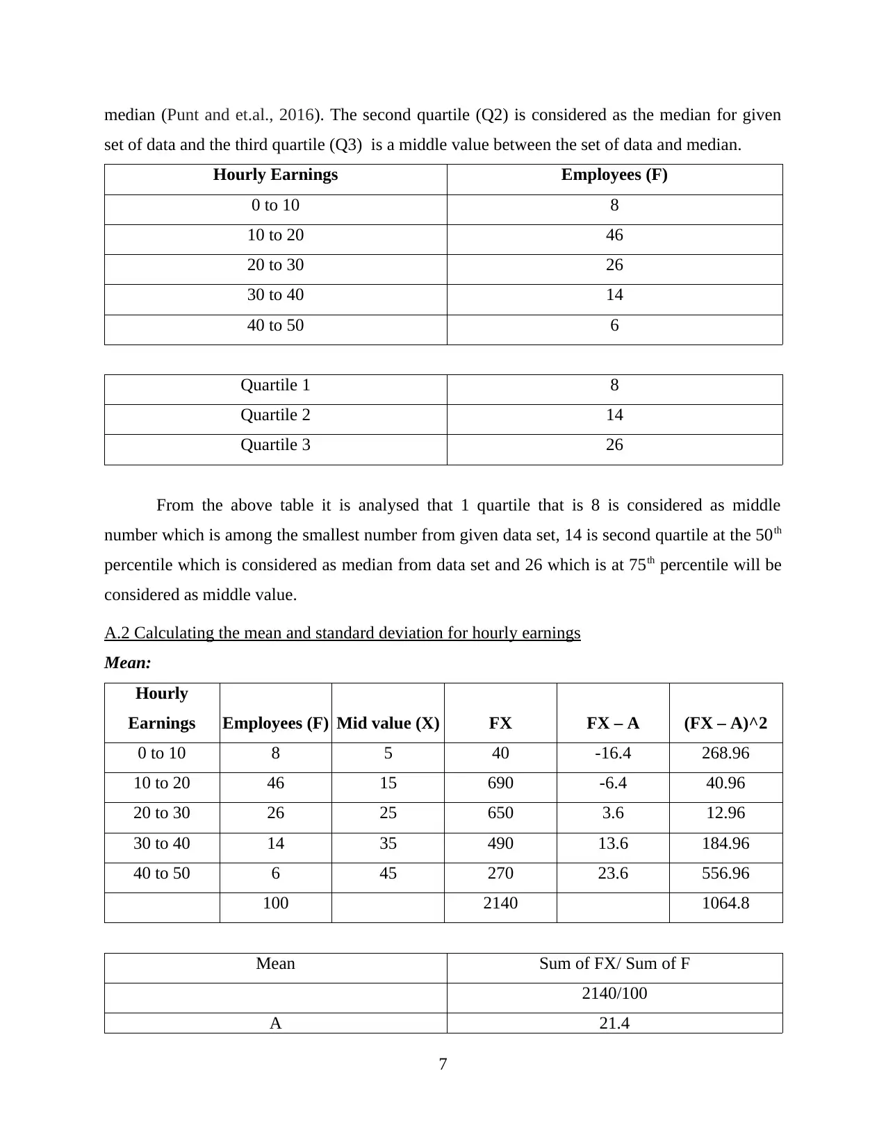
From the above table it is analysed that 1 quartile that is 8 is considered as middle
number which is among the smallest number from given data set, 14 is second quartile at the 50th
percentile which is considered as median from data set and 26 which is at 75th percentile will be
considered as middle value.
A.2 Calculating the mean and standard deviation for hourly earnings
Mean:
Hourly
Earnings Employees (F) Mid value (X) FX FX – A (FX – A)^2
0 to 10 8 5 40 -16.4 268.96
10 to 20 46 15 690 -6.4 40.96
20 to 30 26 25 650 3.6 12.96
30 to 40 14 35 490 13.6 184.96
40 to 50 6 45 270 23.6 556.96
100 2140 1064.8
Mean Sum of FX/ Sum of F
2140/100
A 21.4
7
set of data and the third quartile (Q3) is a middle value between the set of data and median.
Hourly Earnings Employees (F)
0 to 10 8
10 to 20 46
20 to 30 26
30 to 40 14
40 to 50 6
Quartile 1 8
Quartile 2 14
Quartile 3 26
From the above table it is analysed that 1 quartile that is 8 is considered as middle
number which is among the smallest number from given data set, 14 is second quartile at the 50th
percentile which is considered as median from data set and 26 which is at 75th percentile will be
considered as middle value.
A.2 Calculating the mean and standard deviation for hourly earnings
Mean:
Hourly
Earnings Employees (F) Mid value (X) FX FX – A (FX – A)^2
0 to 10 8 5 40 -16.4 268.96
10 to 20 46 15 690 -6.4 40.96
20 to 30 26 25 650 3.6 12.96
30 to 40 14 35 490 13.6 184.96
40 to 50 6 45 270 23.6 556.96
100 2140 1064.8
Mean Sum of FX/ Sum of F
2140/100
A 21.4
7
Paraphrase This Document
Need a fresh take? Get an instant paraphrase of this document with our AI Paraphraser
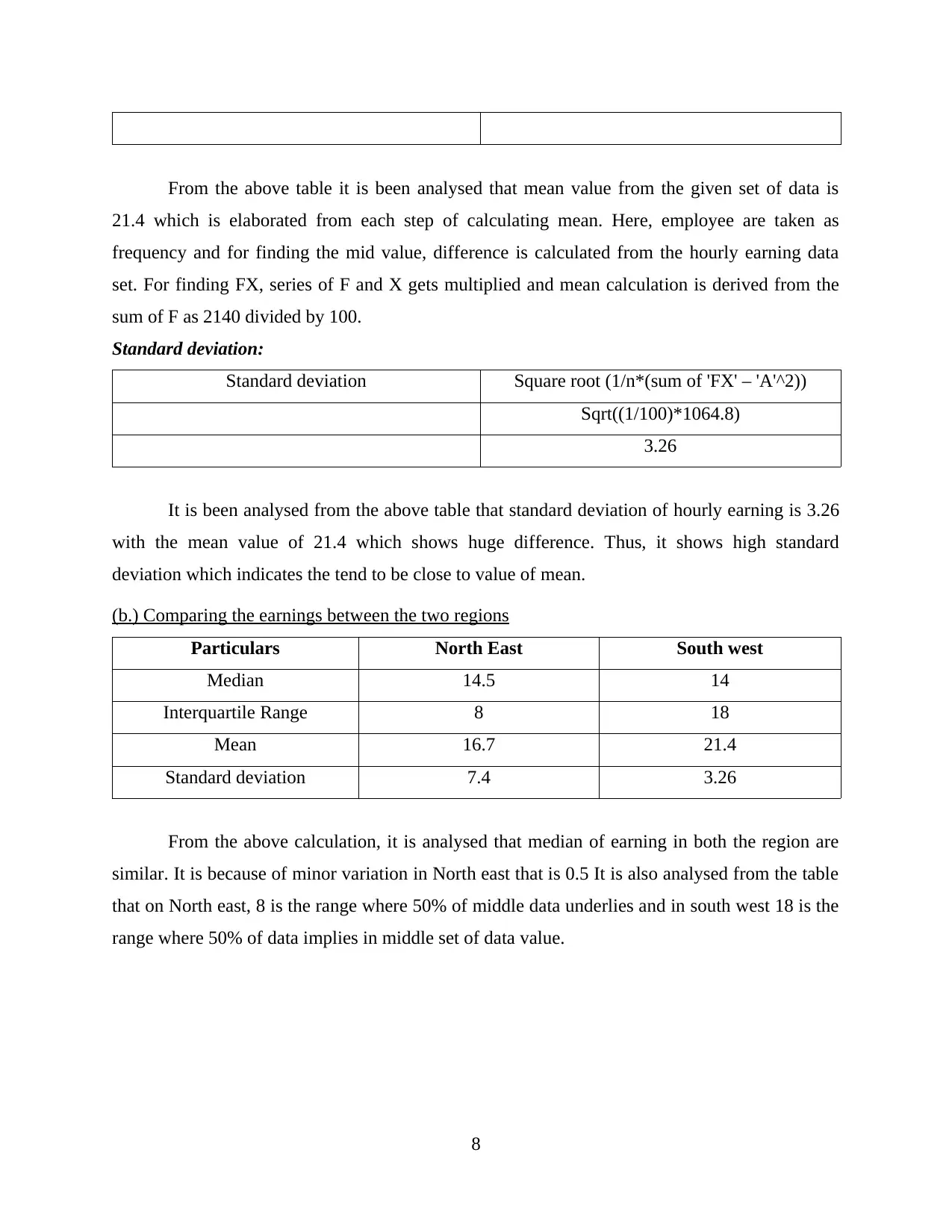
From the above table it is been analysed that mean value from the given set of data is
21.4 which is elaborated from each step of calculating mean. Here, employee are taken as
frequency and for finding the mid value, difference is calculated from the hourly earning data
set. For finding FX, series of F and X gets multiplied and mean calculation is derived from the
sum of F as 2140 divided by 100.
Standard deviation:
Standard deviation Square root (1/n*(sum of 'FX' – 'A'^2))
Sqrt((1/100)*1064.8)
3.26
It is been analysed from the above table that standard deviation of hourly earning is 3.26
with the mean value of 21.4 which shows huge difference. Thus, it shows high standard
deviation which indicates the tend to be close to value of mean.
(b.) Comparing the earnings between the two regions
Particulars North East South west
Median 14.5 14
Interquartile Range 8 18
Mean 16.7 21.4
Standard deviation 7.4 3.26
From the above calculation, it is analysed that median of earning in both the region are
similar. It is because of minor variation in North east that is 0.5 It is also analysed from the table
that on North east, 8 is the range where 50% of middle data underlies and in south west 18 is the
range where 50% of data implies in middle set of data value.
8
ACTIVITY 3 (LO 3)- CLIENT C
1. Stating a suitable hypothesis for testing the claim
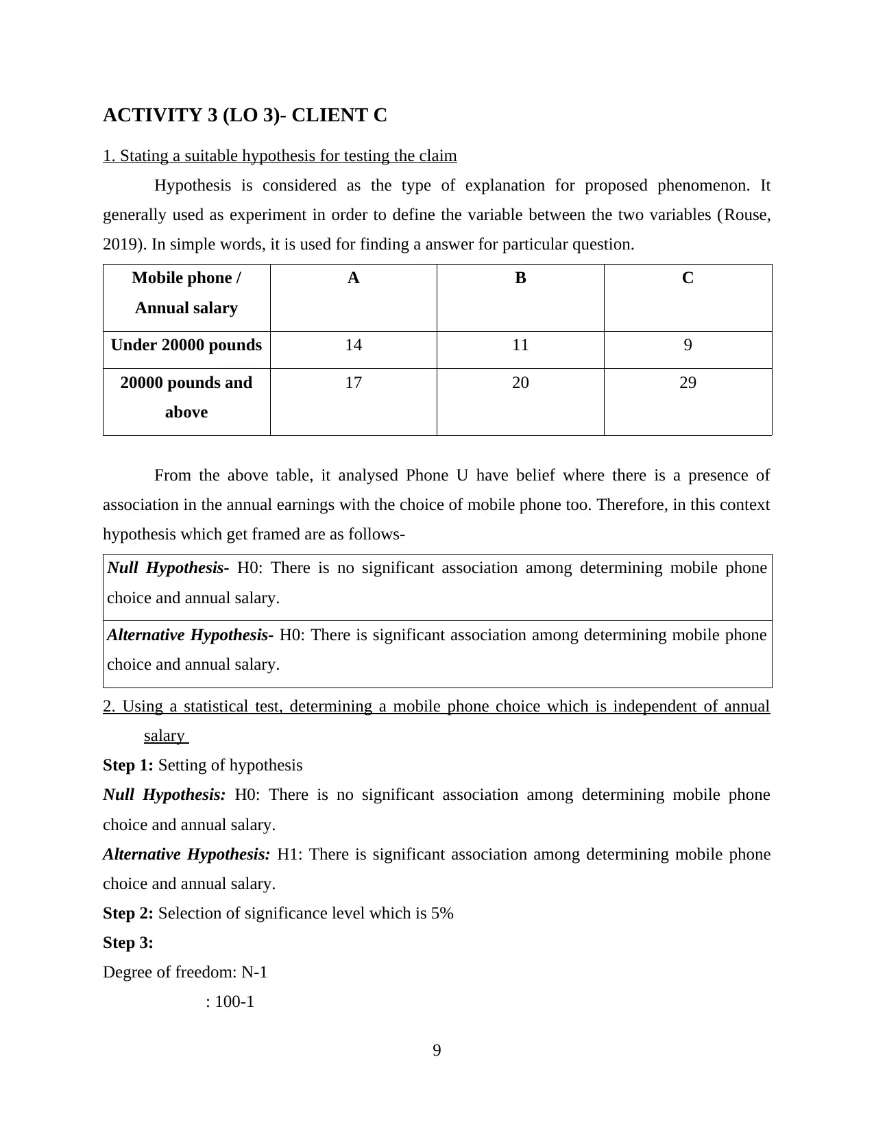
Hypothesis is considered as the type of explanation for proposed phenomenon. It
generally used as experiment in order to define the variable between the two variables (Rouse,
2019). In simple words, it is used for finding a answer for particular question.
Mobile phone /
Annual salary
A B C
Under 20000 pounds 14 11 9
20000 pounds and
above
17 20 29
From the above table, it analysed Phone U have belief where there is a presence of
association in the annual earnings with the choice of mobile phone too. Therefore, in this context
hypothesis which get framed are as follows-
Null Hypothesis- H0: There is no significant association among determining mobile phone
choice and annual salary.
Alternative Hypothesis- H0: There is significant association among determining mobile phone
choice and annual salary.
2. Using a statistical test, determining a mobile phone choice which is independent of annual
salary
Step 1: Setting of hypothesis
Null Hypothesis: H0: There is no significant association among determining mobile phone
choice and annual salary.
Alternative Hypothesis: H1: There is significant association among determining mobile phone
choice and annual salary.
Step 2: Selection of significance level which is 5%
Step 3:
Degree of freedom: N-1
: 100-1
9
1. Stating a suitable hypothesis for testing the claim
Hypothesis is considered as the type of explanation for proposed phenomenon. It
generally used as experiment in order to define the variable between the two variables (Rouse,
2019). In simple words, it is used for finding a answer for particular question.
Mobile phone /
Annual salary
A B C
Under 20000 pounds 14 11 9
20000 pounds and
above
17 20 29
From the above table, it analysed Phone U have belief where there is a presence of
association in the annual earnings with the choice of mobile phone too. Therefore, in this context
hypothesis which get framed are as follows-
Null Hypothesis- H0: There is no significant association among determining mobile phone
choice and annual salary.
Alternative Hypothesis- H0: There is significant association among determining mobile phone
choice and annual salary.
2. Using a statistical test, determining a mobile phone choice which is independent of annual
salary
Step 1: Setting of hypothesis
Null Hypothesis: H0: There is no significant association among determining mobile phone
choice and annual salary.
Alternative Hypothesis: H1: There is significant association among determining mobile phone
choice and annual salary.
Step 2: Selection of significance level which is 5%
Step 3:
Degree of freedom: N-1
: 100-1
9
⊘ This is a preview!⊘
Do you want full access?
Subscribe today to unlock all pages.
Trusted by 1+ million students worldwide
1 out of 15
Related Documents


Your All-in-One AI-Powered Toolkit for Academic Success.
+13062052269
info@desklib.com
Available 24*7 on WhatsApp / Email
![[object Object]](/_next/static/media/star-bottom.7253800d.svg)
Unlock your academic potential
Copyright © 2020–2026 A2Z Services. All Rights Reserved. Developed and managed by ZUCOL.