Statistics 630: Assignment 9 - Estimation & Confidence Intervals

Verified

Added on  2023/01/13

|10
|1808
|50
Homework Assignment
AI Summary
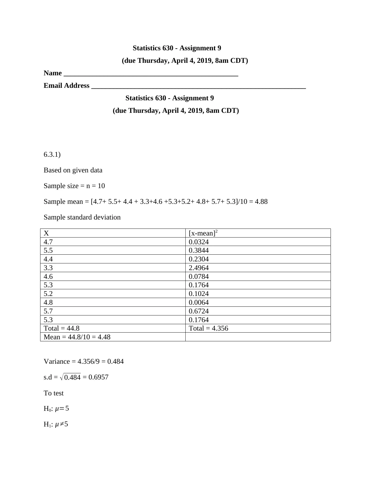
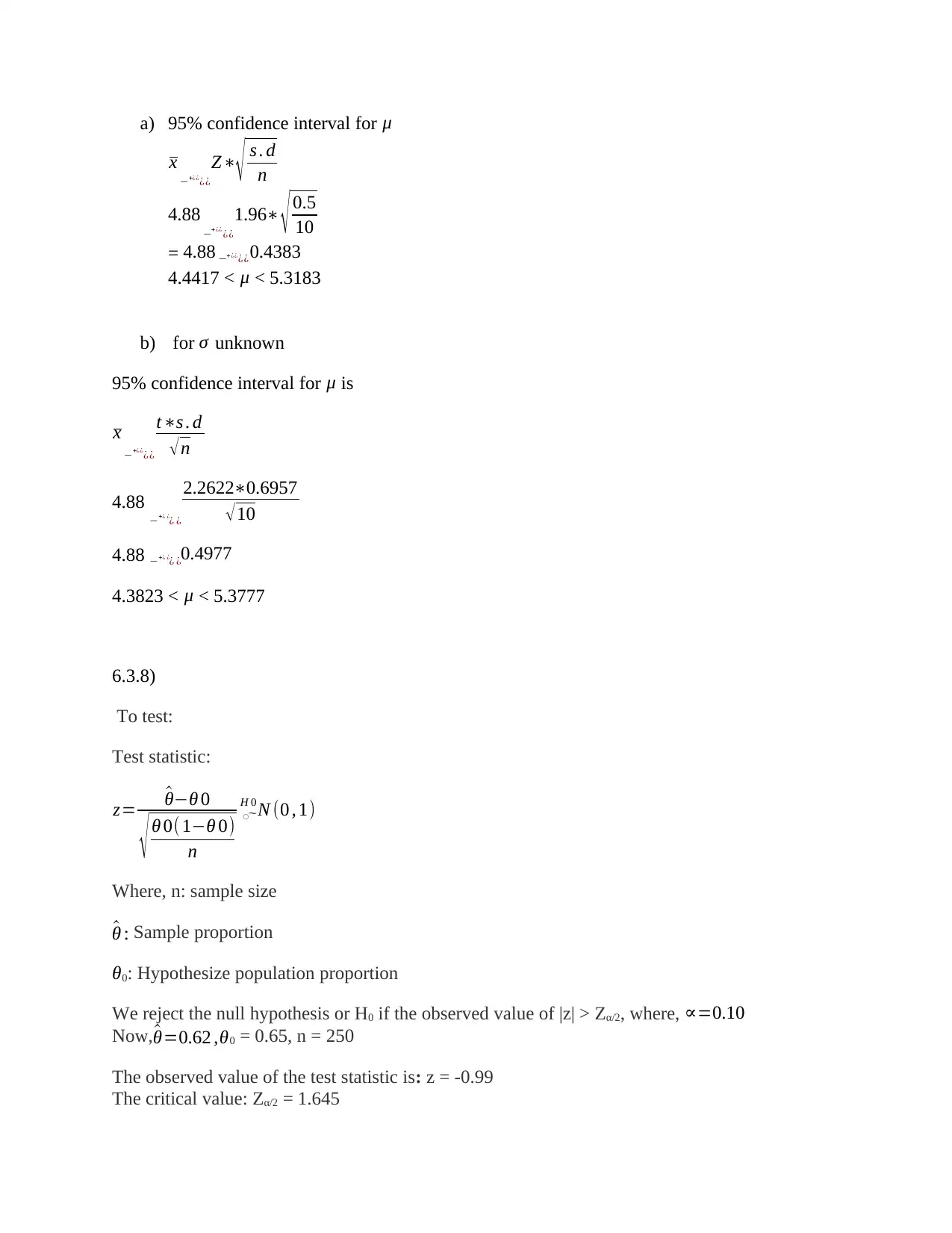
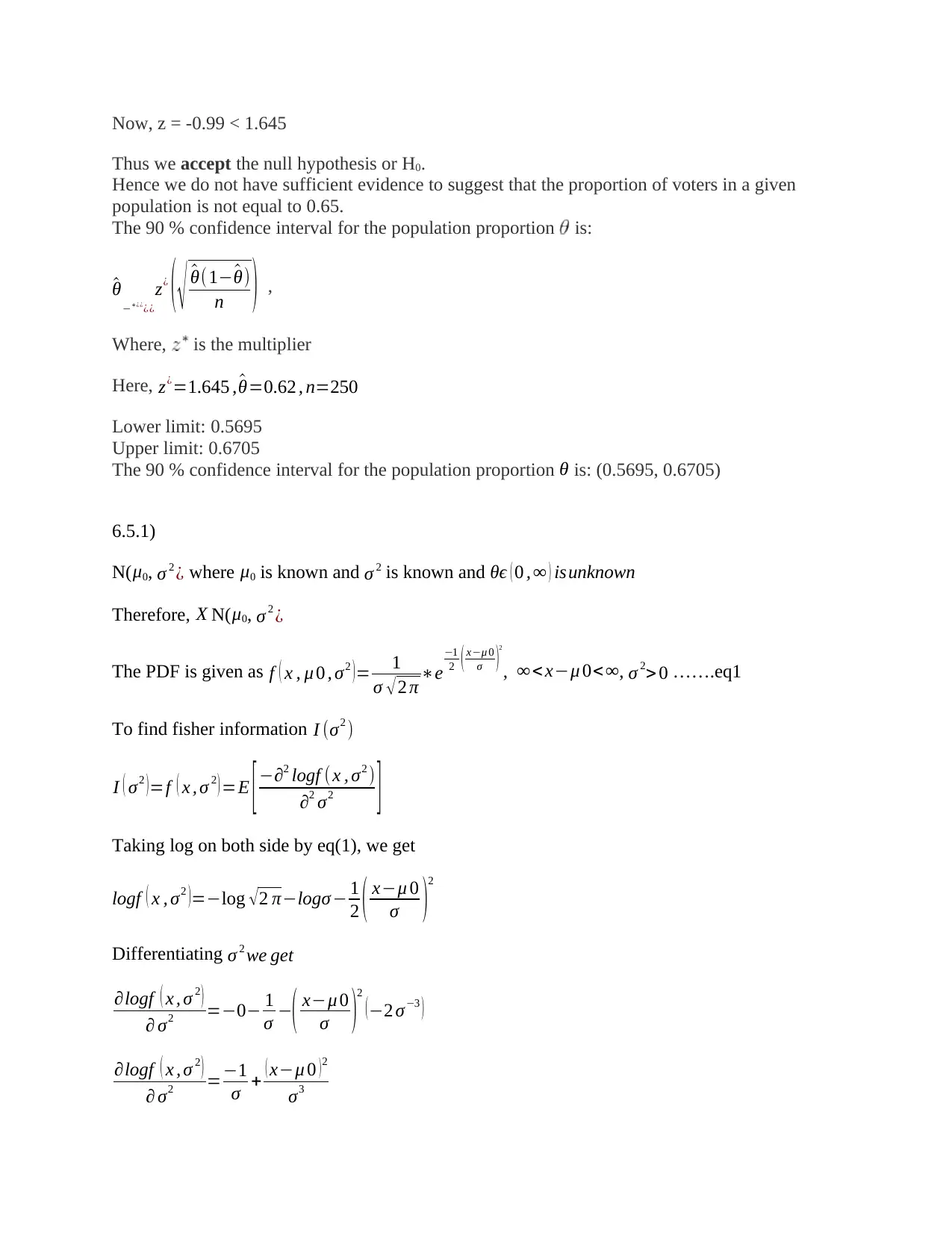
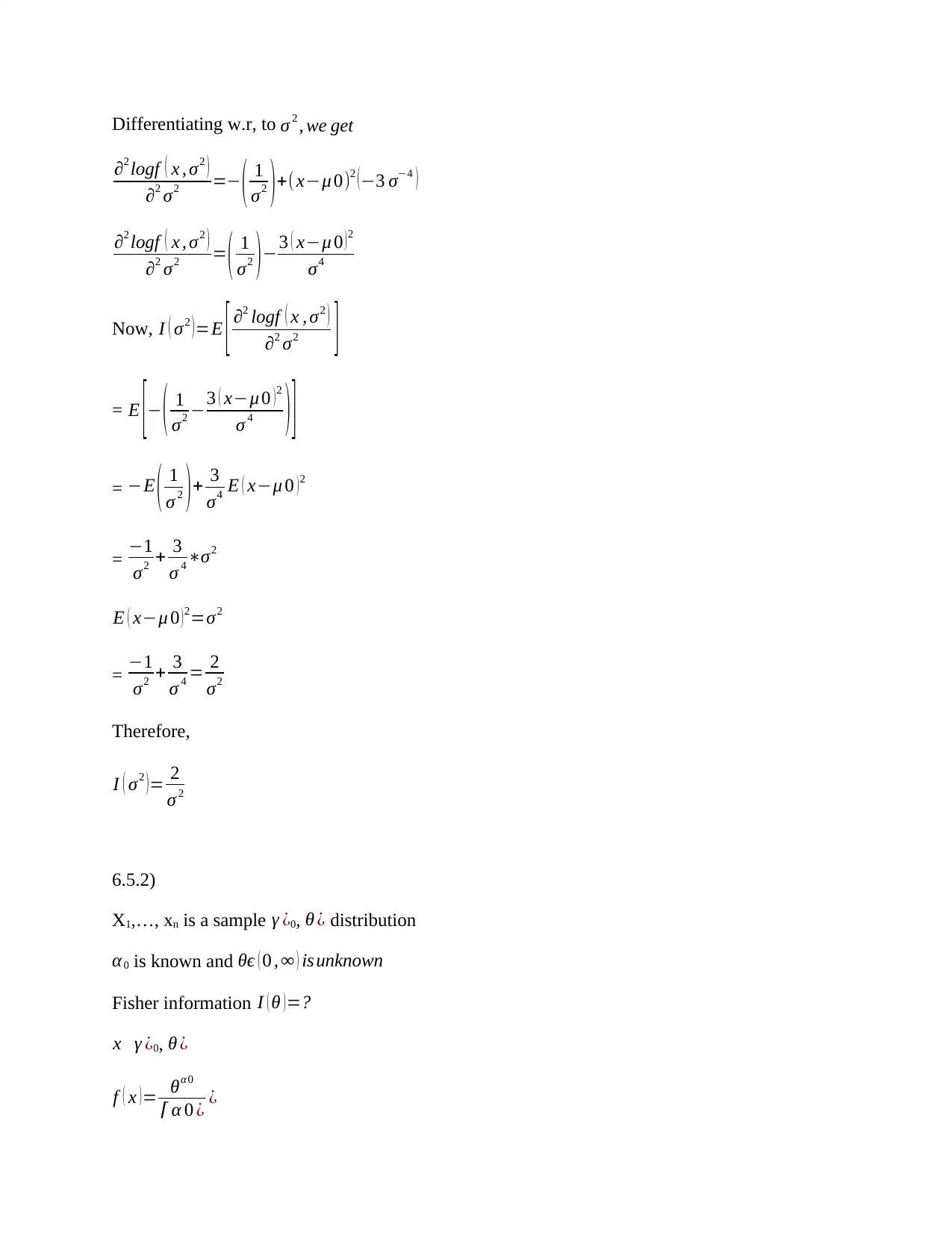
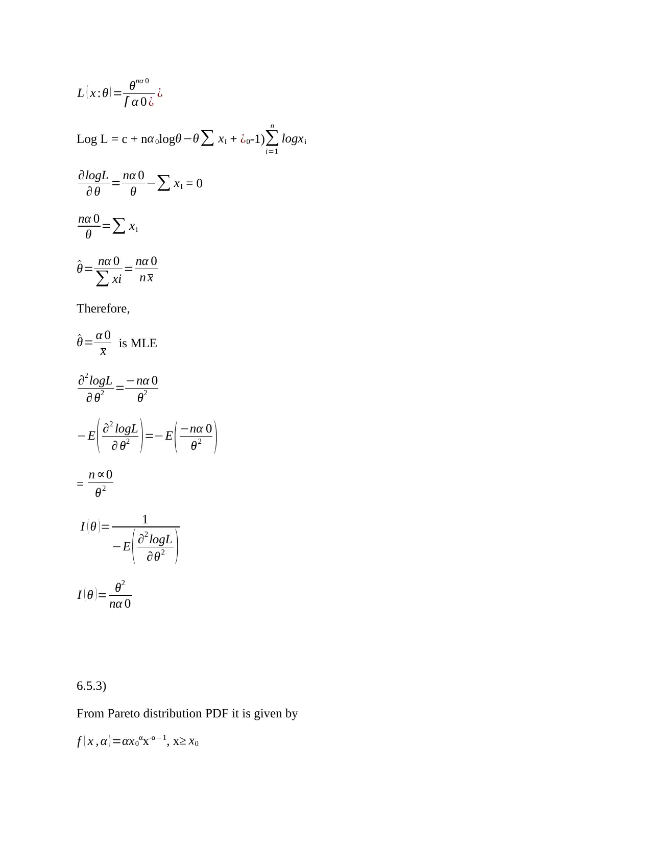
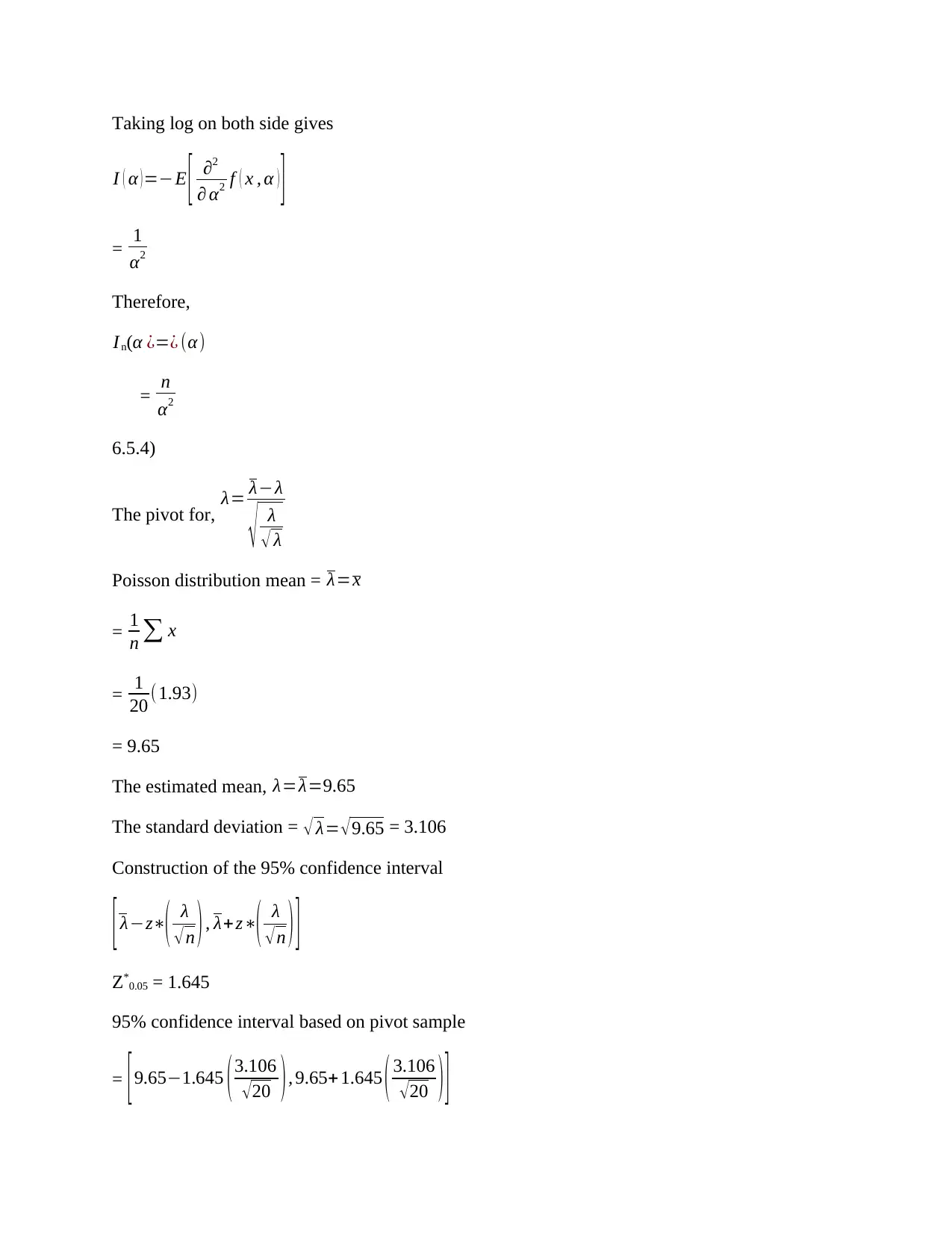
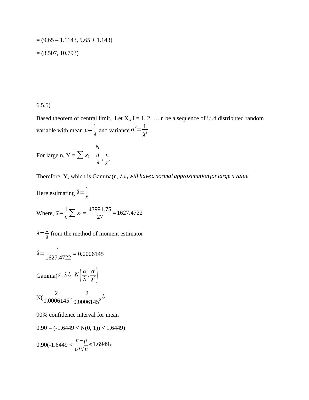
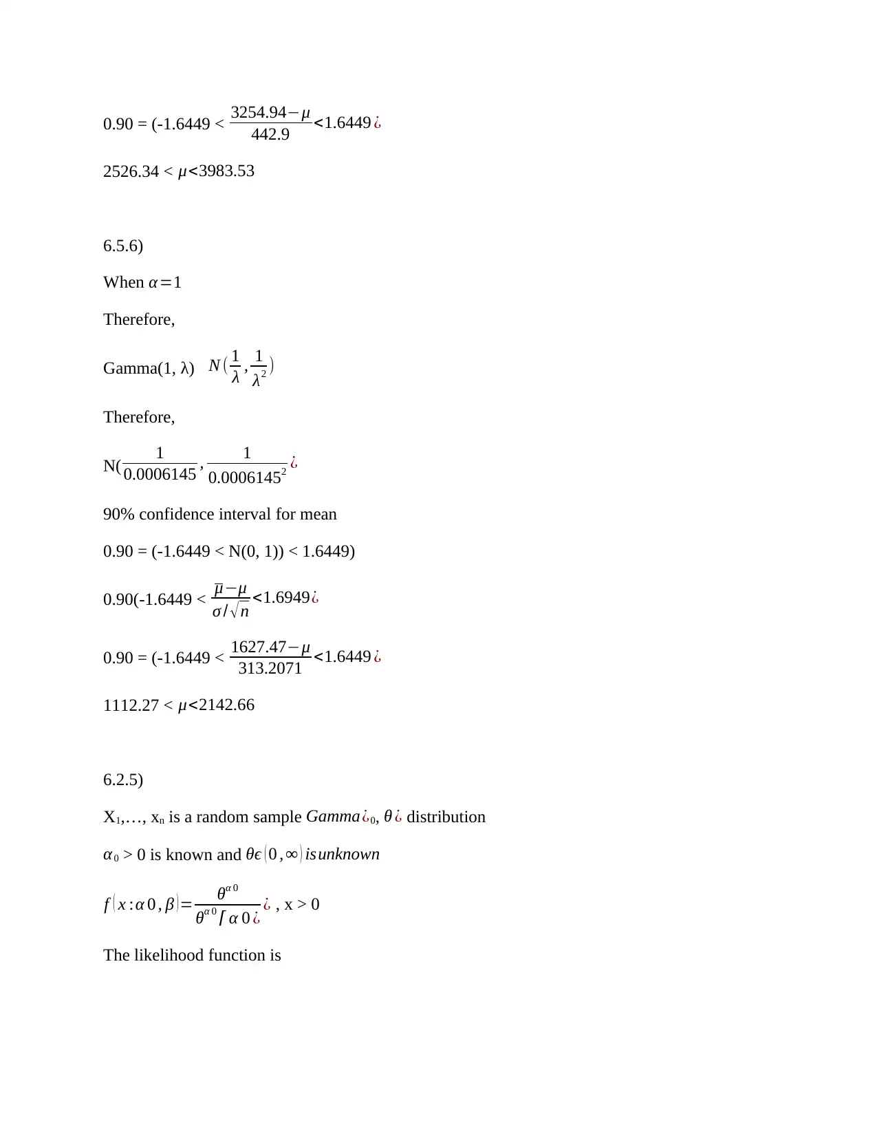
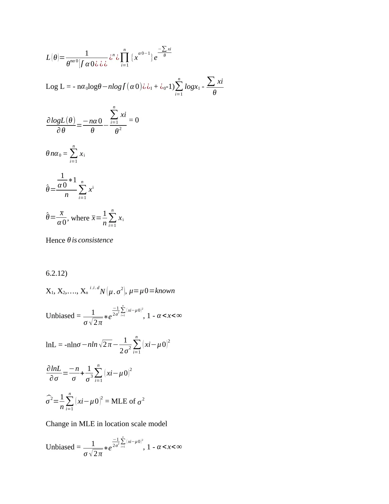
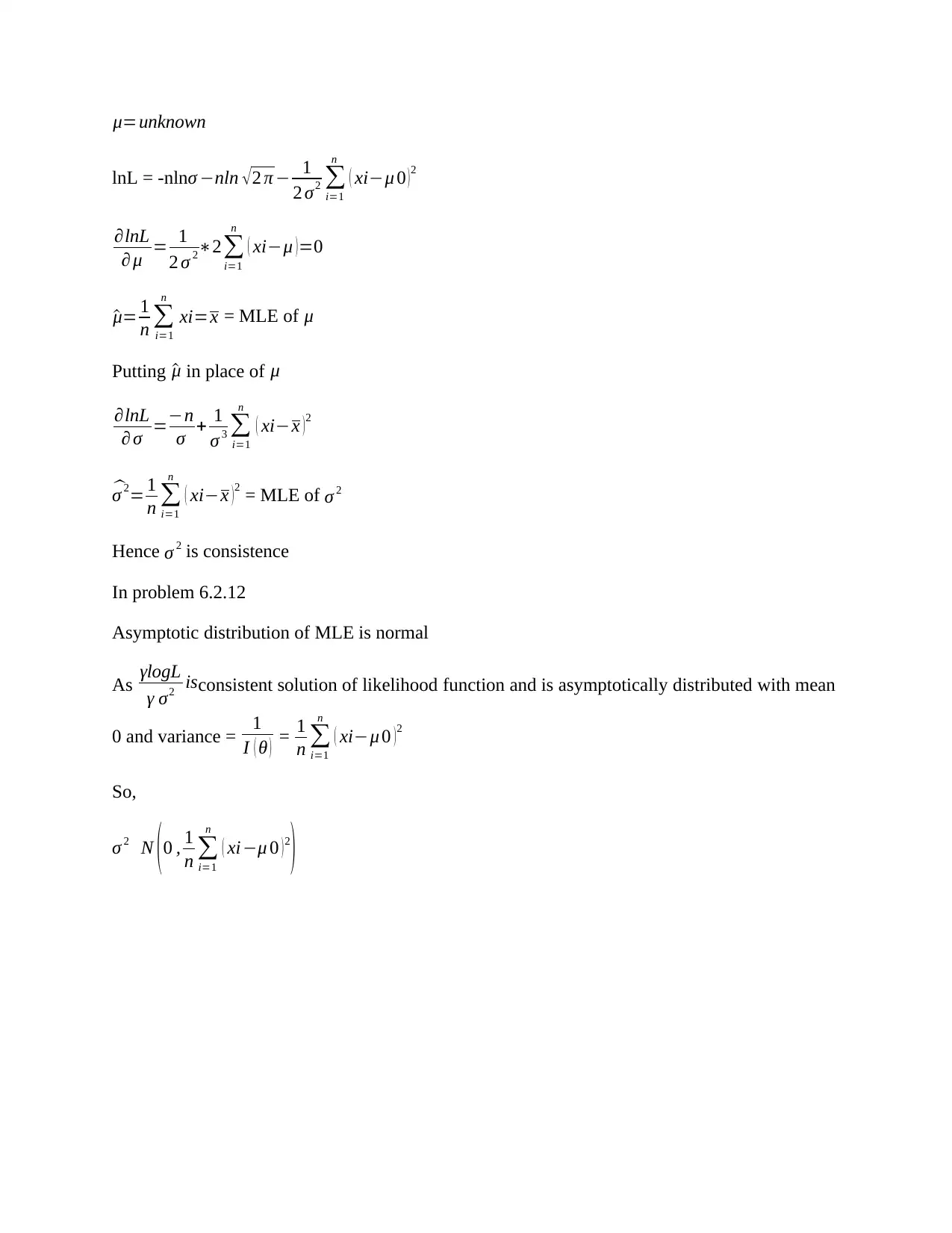
This document presents the complete solutions for Statistics 630 Assignment 9, focusing on key statistical concepts. The assignment covers a range of topics including point estimation, confidence intervals for the mean with known and unknown variance, and hypothesis testing using the Z-test. Further, it delves into Fisher information, maximum likelihood estimation (MLE), and the properties of estimators. The solutions also address confidence intervals for population proportions, Fisher information for different distributions (normal, gamma, Pareto), and applications of the Poisson distribution and the Central Limit Theorem. Detailed calculations and explanations are provided for each problem, including the construction of confidence intervals using pivots and the application of the method of moments estimator.
tabler-icon-diamond-filled.svg

Contribute Materials

Your contribution can guide someone’s learning journey. Share your documents today.
Document Page
Statistics 630 - Assignment 9
(due Thursday, April 4, 2019, 8am CDT)
Name ________________________________________________
Email Address ___________________________________________________________
Statistics 630 - Assignment 9
(due Thursday, April 4, 2019, 8am CDT)
6.3.1)
Based on given data
Sample size = n = 10
Sample mean = [4.7+ 5.5+ 4.4 + 3.3+4.6 +5.3+5.2+ 4.8+ 5.7+ 5.3]/10 = 4.88
Sample standard deviation
X [x-mean]2
4.7 0.0324
5.5 0.3844
4.4 0.2304
3.3 2.4964
4.6 0.0784
5.3 0.1764
5.2 0.1024
4.8 0.0064
5.7 0.6724
5.3 0.1764
Total = 44.8 Total = 4.356
Mean = 44.8/10 = 4.48
Variance = 4.356/9 = 0.484
s.d = 0.484 = 0.6957
To test
H0: μ=5
H1: μ 5
tabler-icon-diamond-filled.svg

Secure Best Marks with AI Grader

Need help grading? Try our AI Grader for instant feedback on your assignments.
Document Page
a) 95% confidence interval for μ
x Z
s . d
n ¿
+¿¿ ¿
4.88 1.96 0.5
10 ¿
+ ¿¿ ¿
= 4.88 0.4383 ¿+ ¿¿ ¿
4.4417 < μ < 5.3183
b) for σ unknown
95% confidence interval for μ is
x ts . d
n ¿
+¿¿ ¿
4.88 2.26220.6957
10 ¿
+¿ ¿ ¿
4.88 0.4977 ¿+¿ ¿ ¿
4.3823 < μ < 5.3777
6.3.8)
To test:
Test statistic:
z= ^θθ 0
θ 0( 1θ 0)
n
N (0 , 1)͠
H 0
Where, n: sample size
^θ : Sample proportion
θ0: Hypothesize population proportion
We reject the null hypothesis or H0 if the observed value of |z| > Zα/2, where, =0.10
Now, ^θ=0.62 ,θ0 = 0.65, n = 250
The observed value of the test statistic is: z = -0.99
The critical value: Zα/2 = 1.645
Document Page
Now, z = -0.99 < 1.645
Thus we accept the null hypothesis or H0.
Hence we do not have sufficient evidence to suggest that the proportion of voters in a given
population is not equal to 0.65.
The 90 % confidence interval for the population proportion is:
^θ z¿
( ^θ(1 ^θ)
n ) ¿
+ ¿¿ ¿
,
Where, is the multiplier
Here, z¿=1.645 , ^θ=0.62 , n=250
Lower limit: 0.5695
Upper limit: 0.6705
The 90 % confidence interval for the population proportion θ is: (0.5695, 0.6705)
6.5.1)
N( μ0, σ 2 ¿ where μ0 is known and σ 2 is known and θϵ ( 0 , ) isunknown
Therefore, X N( μ0, σ 2 ¿
The PDF is given as f ( x , μ 0 , σ2 )= 1
σ 2 π e
1
2 ( xμ 0
σ )
2
, <xμ 0< , σ 2> 0 …….eq1
To find fisher information I (σ2 )
I ( σ2 ) =f ( x , σ 2 ) =E [ 2 logf ( x , σ2 )
2 σ2 ]
Taking log on both side by eq(1), we get
logf ( x , σ2 )=log 2 πlogσ 1
2 ( xμ 0
σ )
2
Differentiating σ 2 we get
logf ( x , σ 2 )
σ2 =0 1
σ ( xμ 0
σ )2
(2 σ3 )
logf ( x , σ 2 )
σ2 =1
σ + ( xμ 0 ) 2
σ3
Document Page
Differentiating w.r, to σ 2 , we get
2 logf ( x , σ2 )
2 σ2 = ( 1
σ2 ) +( xμ 0)2 ( 3 σ4 )
2 logf ( x , σ2 )
2 σ2 = ( 1
σ2 ) 3 ( xμ 0 ) 2
σ4
Now, I ( σ2 )=E [ 2 logf ( x , σ2 )
2 σ2 ]
= E [ ( 1
σ2 3 ( xμ 0 )2
σ 4 ) ]
= E ( 1
σ 2 )+ 3
σ4 E ( xμ 0 )2
= 1
σ2 + 3
σ 4 σ2
E ( xμ 0 )2=σ2
= 1
σ2 + 3
σ 4 = 2
σ2
Therefore,
I ( σ2 )= 2
σ 2
6.5.2)
X1,…, xn is a sample γ ¿0, θ ¿ distribution
α0 is known and θϵ ( 0 , ) isunknown
Fisher information I ( θ )=?
x γ ¿0, θ ¿
f ( x )= θα 0
α 0 ¿ ¿
tabler-icon-diamond-filled.svg

Secure Best Marks with AI Grader

Need help grading? Try our AI Grader for instant feedback on your assignments.
Document Page
L ( x :θ ) = θ 0
α 0 ¿ ¿
Log L = c + n α 0log θθ xI + ¿0-1)
i=1
n
logxi
logL
θ = 0
θ xI = 0
0
θ = xi
^θ= 0
xi = 0
n x
Therefore,
^θ= α 0
x is MLE
2 logL
θ2 = 0
θ2
E ( 2 logL
θ2 ) =E ( 0
θ2 )
= n 0
θ2
I ( θ )= 1
E ( 2 logL
θ2 )
I ( θ ) = θ2
0
6.5.3)
From Pareto distribution PDF it is given by
f ( x , α ) =αx0αx-α – 1, x x0
Document Page
Taking log on both side gives
I ( α ) =E [ 2
α2 f ( x , α ) ]
= 1
α2
Therefore,
In(α ¿=¿ (α)
= n
α2
6.5.4)
The pivot for, λ= λλ
λ
λ
Poisson distribution mean = λ=x
= 1
n x
= 1
20 (1.93)
= 9.65
The estimated mean, λ=λ=9.65
The standard deviation = λ= 9.65 = 3.106
Construction of the 95% confidence interval
[ λz( λ
n ) , λ+ z( λ
n ) ]
Z*0.05 = 1.645
95% confidence interval based on pivot sample
= [ 9.651.645 ( 3.106
20 ) , 9.65+ 1.645 ( 3.106
20 ) ]
Document Page
= (9.65 – 1.1143, 9.65 + 1.143)
= (8.507, 10.793)
6.5.5)
Based theorem of central limit, Let Xi, I = 1, 2, … n be a sequence of i.i.d distributed random
variable with mean μ= 1
λ and variance σ 2= 1
λ2
For large n, Y = xI
N
n
λ , n
λ2
Therefore, Y, which is Gamma(n, λ ¿ , will have a normal approximation for large n value
Here estimating ^λ= 1
x
Where, x= 1
n xI = 43991.75
27 =1627.4722
λ= 1
λ from the method of moment estimator
^λ= 1
1627.4722 = 0.0006145
Gamma(α , λ ¿ N ( α
λ , α
λ2 )
N( 2
0.0006145 , 2
0.00061452 ¿
90% confidence interval for mean
0.90 = (-1.6449 < N(0, 1)) < 1.6449)
0.90(-1.6449 < μμ
σ / n <1.6949¿
tabler-icon-diamond-filled.svg

Paraphrase This Document

Need a fresh take? Get an instant paraphrase of this document with our AI Paraphraser
Document Page
0.90 = (-1.6449 < 3254.94μ
442.9 <1.6449 ¿
2526.34 < μ<3983.53
6.5.6)
When α =1
Therefore,
Gamma(1, λ) N ( 1
λ , 1
λ2 )
Therefore,
N( 1
0.0006145 , 1
0.00061452 ¿
90% confidence interval for mean
0.90 = (-1.6449 < N(0, 1)) < 1.6449)
0.90(-1.6449 < μμ
σ / n <1.6949¿
0.90 = (-1.6449 < 1627.47μ
313.2071 <1.6449 ¿
1112.27 < μ<2142.66
6.2.5)
X1,…, xn is a random sample Gamma¿0, θ ¿ distribution
α0 > 0 is known and θϵ ( 0 , ) isunknown
f ( x :α 0 , β )= θα 0
θα 0 α 0 ¿ ¿ , x > 0
The likelihood function is
Document Page
L ( θ ) = 1
θ 0 [ α 0¿ ¿ ¿ ¿n ¿
i=1
n
{xα 01
}e
xi
θ
Log L = - n α0logθnlog ( α 0)¿ ¿I + ¿0-1)
i=1
n
logxI - xi
θ
logL(θ)
θ = 0
θ

i=1
n
xi
θ2
= 0
θ 0 =
i=1
n
xi
^θ=
1
α 0 1
n
i=1
n
xi
^θ= x
α 0 , where x= 1
n
i=1
n
xi
Hence θ is consistence
6.2.12)
X1, X2,…., Xn N ( μ . σ2 )
i .i . d , μ=μ 0=known
Unbiased = 1
σ 2 π e
1
2 σ2
i=1
n
( xiμ 0 ) 2
, 1 - α < x<
lnL = -nlnσ nln 2 π 1
2 σ2
i=1
n
( xiμ 0 )2
lnL
σ =n
σ + 1
σ 3
i=1
n
( xiμ 0 )2
^σ 2= 1
n
i=1
n
( xiμ 0 )2 = MLE of σ 2
Change in MLE in location scale model
Unbiased = 1
σ 2 π e
1
2 σ2
i=1
n
( xiμ 0 ) 2
, 1 - α < x<
Document Page
μ=unknown
lnL = -nlnσ nln 2 π 1
2 σ2
i=1
n
( xiμ 0 )2
lnL
μ = 1
2 σ 22
i=1
n
( xiμ )=0
^μ= 1
n
i=1
n
xi=x = MLE of μ
Putting ^μ in place of μ
lnL
σ =n
σ + 1
σ 3
i=1
n
( xix )2
^σ 2= 1
n
i=1
n
( xix ) 2 = MLE of σ 2
Hence σ 2 is consistence
In problem 6.2.12
Asymptotic distribution of MLE is normal
As γlogL
γ σ2 isconsistent solution of likelihood function and is asymptotically distributed with mean
0 and variance = 1
I ( θ ) = 1
n
i=1
n
( xiμ 0 )2
So,
σ 2 N ( 0 , 1
n
i=1
n
( xiμ 0 ) 2
)
chevron_up_icon
1 out of 10
circle_padding
hide_on_mobile
zoom_out_icon
logo.png

Your All-in-One AI-Powered Toolkit for Academic Success.

Available 24*7 on WhatsApp / Email

[object Object]