University Statistics: Exam 2 - Hypothesis Testing Solutions

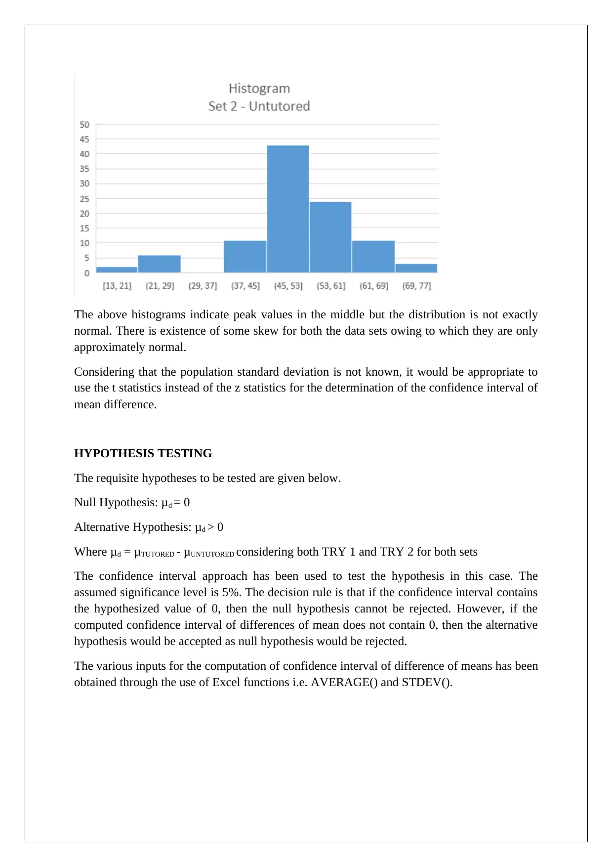
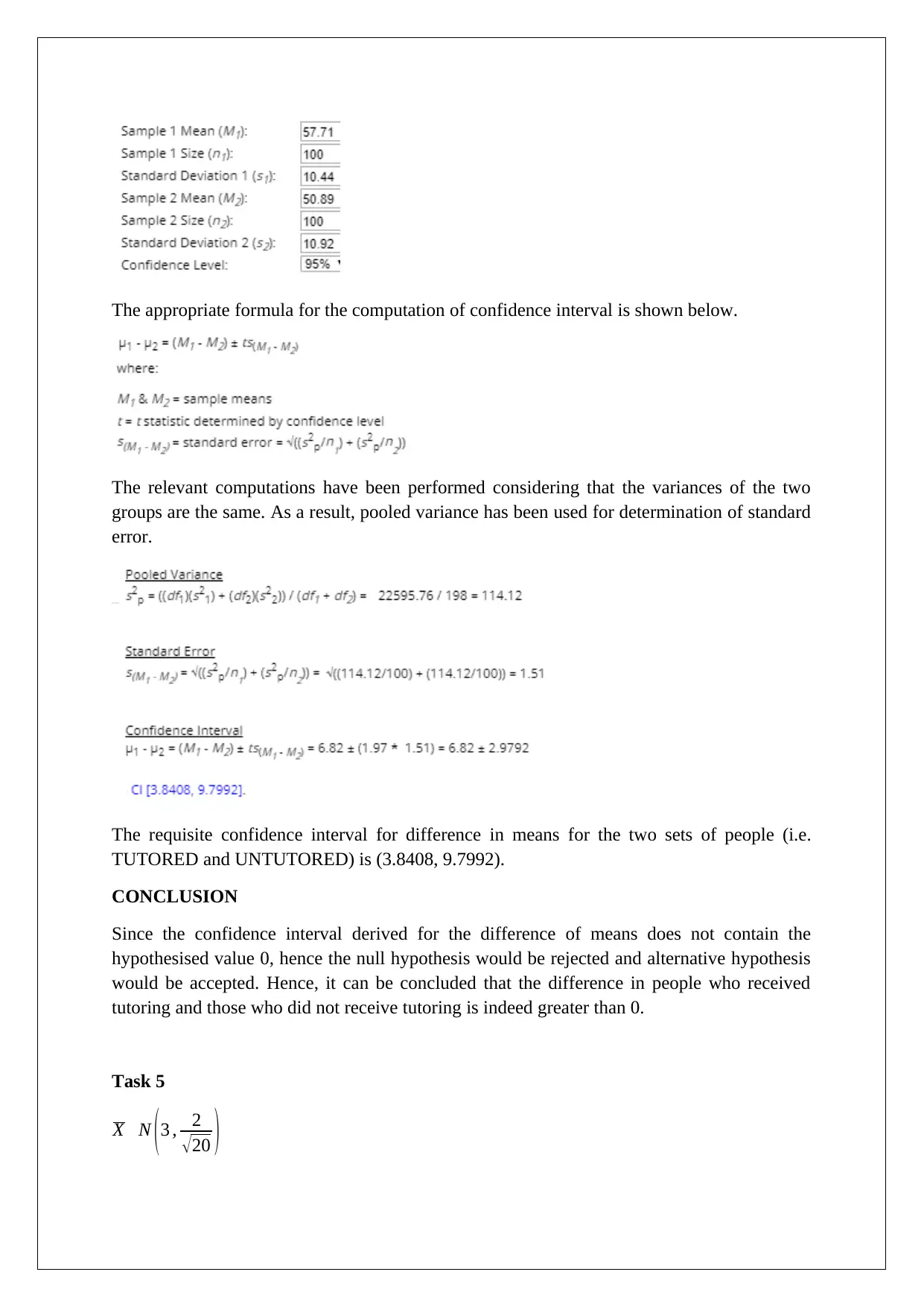
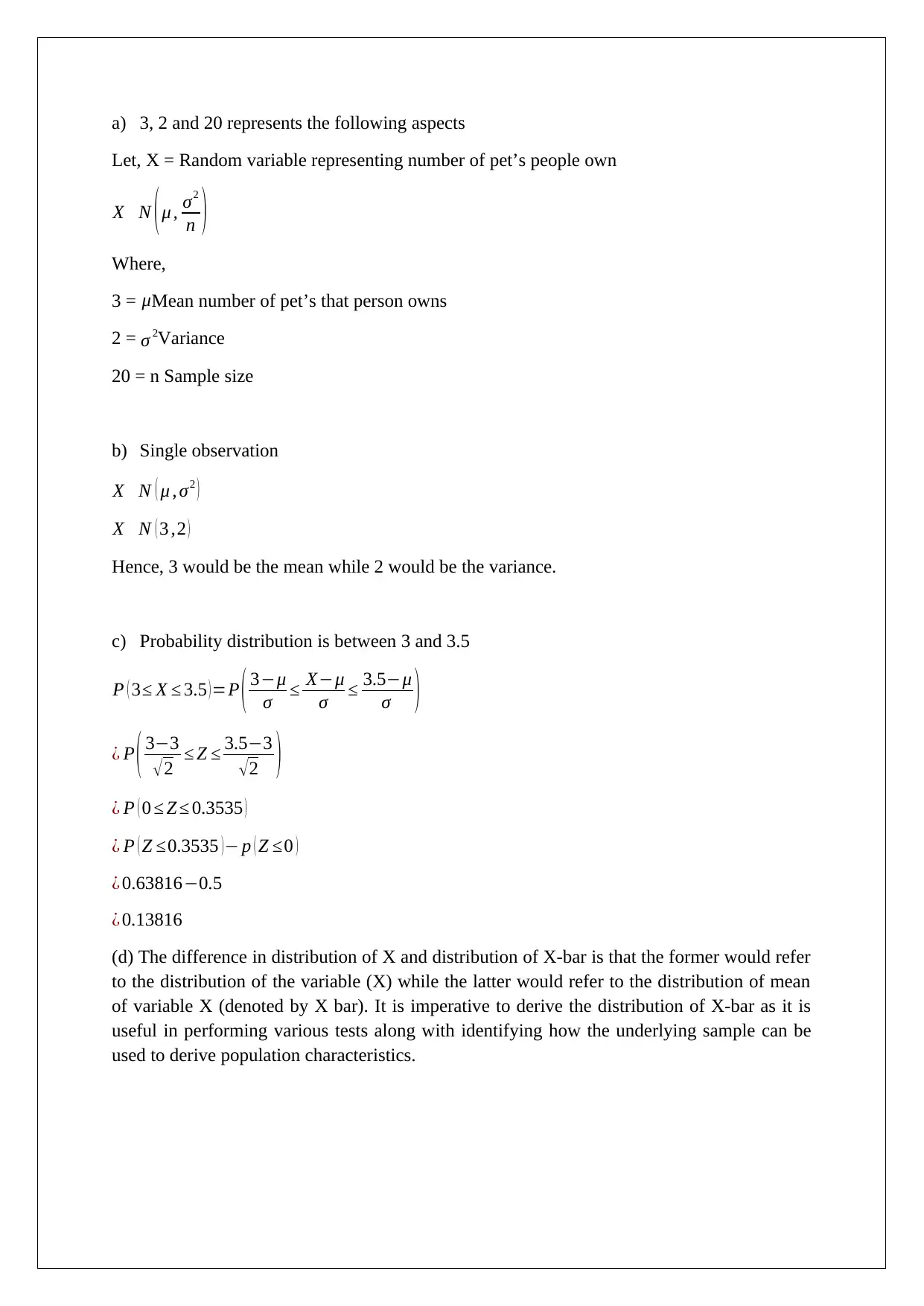
This document presents a comprehensive solution to a statistics exam, addressing five distinct tasks. Task 1 focuses on checking assumptions for a one-sample z-test, performing hypothesis testing, and constructing a 95% confidence interval to determine if the mean stem length of roses differs from 11. Task 2 involves a binomial distribution analysis, checking for normality, performing hypothesis testing using a z-test, and constructing a confidence interval to assess whether more than 80% of the population likes dogs. Tasks 3 and 4 compare two sets of data, employing t-tests and confidence intervals to evaluate the impact of tutoring on performance, considering both tutored and untutored groups. Finally, Task 5 interprets statistical parameters (mean, variance, sample size) and discusses the difference between the distribution of a variable and the distribution of its mean. The solutions include detailed explanations, Excel computations, and conclusions based on p-values and confidence intervals.

BASIC PRACTICE OF STATISTICS
STUDENT ID:
[Pick the date]

Task 1
Checking Assumptions
Since there is no explicit mention of the underlying sampling, hence an SRS has been
assumed. Further, the histogram of the given data has been obtained in order to check if the
distribution of the sample data can be assumed to be normal or not.
Based on the above histogram, it can be assumed that the underlying data is normally
distributed since it is almost symmetric. Additionally, central limit theorem also states that if
the underlying sample size is greater than 30, then the underlying sample can be assumed as
normally distributed. Since, the sample size is greater than 30, normality of sample can also
be established from this theorem.
Further, it is noteworthy that the population standard deviation has been given which implies
that the appropriate test statistics would be z and not t. T is a suitable test statistic when
population standard deviation is unknown and also the sample size is small. Hence, one
sample z test would be used here.
TESTING HYPOTHESIS
The sample mean has been determined using Excel functions for average. Sample mean =
11.8875
Standard error = 3/5000.5 = 0.1342
The requisite hypotheses for the given problem are mentioned below.
Null hypothesis H0 :μ=11 i.e. average stem length of rose is 11.
Alternative hypothesis Ha : μ ≠11 i. e . stem length of roseis not 11.

Z= x −μ0
s / √n
Putting the input values obtained above, we get z = (11.8875-11)/0.1342 = 6.15
The corresponding p value for the above z value is 0.
The requisite 95% confidence interval for the mean has been computed using Excel and
relevant screenshot is provided below.
Hence, the requisite confidence interval is (11.639,12.136).
CONCLUSION
Since p value is less than assumed significance level of 1%, hence the null hypothesis would
be rejected and alternative hypothesis would be accepted. Hence, the conclusion is that mean
stem lengths of roses is different from 11. Since the confidence interval does not include 11,
hence the average length of stem of roses for population exceeds 11.
Task 2
Checking Assumptions
The given distribution is binomial considering that there are only two alternatives to choose
from i.e. Yes and NO. Also, each of the responses are independent from each other. In order
to test hypothesis, we need to test whether the underlying binomial distribution can be
considered as normal distribution.
For the above to happen, following conditions ought to be satisfied.
np ≥ 5
np(1-p) ≥ 5

where n = number of trials
and p = probability of success
In the given case, n = 500, p = 0.84
n*p = 500*0.84 = 420
np(1-p) = 500*84*0.16 = 67.2
Clearly, both the above terms are greater than 5 owing to which the given binomial
distribution can be approximated as normal distribution. Thus, the appropriate test statistics
for testing of hypothesis would be Z.
TESTING HYPOTHESIS
The requisite hypotheses are as stated below.
Null Hypothesis: p = 0.8 i.e. only 80% of the population like dogs
Alternative Hypothesis: p > 0.8 i.e. more than 80% of the population like dogs
The hypothesis testing can be performed using the test statistic and also using the confidence
interval approach. Both have been carried out below.
The requisite formula to be used is given below.
The above computations have been performed in Excel and respective p value has been
found. It has come out as 0.0127. The relevant screenshot is shown below.

The requisite confidence interval computations have been performed in Excel and pasted
below.
CONCLUSION
Based on the above hypothesis testing, assuming a level of significance of 5%, the null
hypothesis can be rejected as the p value is lower than 5%. The 95% confidence interval for
population proportion also supports this conclusion since both the lower and upper end of
confidence intervals are greater than 0.8.
Task 3
Checking Assumptions
The first assumption is check relates to the distribution of the two variables to be considered
here. These are TRY 1(Set 1) and TRY 2 (Set 2).
The requisite histograms are shown as follows.

The above histograms indicate peak values in the middle but the distribution is not exactly
normal. There is existence of some skew for both the data sets owing to which they are only
approximately normal.
Considering that the population standard deviation is not known, it would be appropriate to
use the t statistics instead of the z statistics for the determination of the confidence interval of
mean difference.

HYPOTHESIS TESTING
The requisite hypotheses to be tested are given below.
Null Hypothesis: μd = 0
Alternative Hypothesis: μd > 0
Where μd = μTRY2 - μTRY1 considering only tutored people
The confidence interval approach has been used to test the hypothesis in this case. The
assumed significance level is 5%. The decision rule is that if the confidence interval contains
the hypothesized value of 0, then the null hypothesis cannot be rejected. However, if the
computed confidence interval of differences of mean does not contain 0, then the alternative
hypothesis would be accepted as null hypothesis would be rejected.
The various inputs for the computation of confidence interval of difference of means has been
obtained through the use of Excel functions i.e. AVERAGE() and STDEV().
The appropriate formula for the computation of confidence interval is shown below.
The relevant computations have been performed considering that the variances of the two
groups are the same. As a result, pooled variance has been used for determination of standard
error.
Degrees of freedom for t = 50+50-2 = 98

The requisite confidence interval for difference in means for the two sets of people who were
tutored is (3.4862, 11.2738).
CONCLUSION
Since the confidence interval derived for the difference of means does not contain the
hypothesised value 0, hence the null hypothesis would be rejected and alternative hypothesis
would be accepted. Hence, it can be concluded that the difference in people who received
tutoring is indeed greater than 0.
Task 4
Checking Assumptions
The first assumption is check relates to the distribution of the two variables to be considered
here. These are SET 1:TUTORED (Total 100 observations i.e. TRY 1+ TRY 2) and Set 2:
UNTUTORED (Total 100 observations i.e. TRY 1+ TRY 2).
The requisite histograms are shown as follows.

The above histograms indicate peak values in the middle but the distribution is not exactly
normal. There is existence of some skew for both the data sets owing to which they are only
approximately normal.
Considering that the population standard deviation is not known, it would be appropriate to
use the t statistics instead of the z statistics for the determination of the confidence interval of
mean difference.
HYPOTHESIS TESTING
The requisite hypotheses to be tested are given below.
Null Hypothesis: μd = 0
Alternative Hypothesis: μd > 0
Where μd = μTUTORED - μUNTUTORED considering both TRY 1 and TRY 2 for both sets
The confidence interval approach has been used to test the hypothesis in this case. The
assumed significance level is 5%. The decision rule is that if the confidence interval contains
the hypothesized value of 0, then the null hypothesis cannot be rejected. However, if the
computed confidence interval of differences of mean does not contain 0, then the alternative
hypothesis would be accepted as null hypothesis would be rejected.
The various inputs for the computation of confidence interval of difference of means has been
obtained through the use of Excel functions i.e. AVERAGE() and STDEV().

The appropriate formula for the computation of confidence interval is shown below.
The relevant computations have been performed considering that the variances of the two
groups are the same. As a result, pooled variance has been used for determination of standard
error.
The requisite confidence interval for difference in means for the two sets of people (i.e.
TUTORED and UNTUTORED) is (3.8408, 9.7992).
CONCLUSION
Since the confidence interval derived for the difference of means does not contain the
hypothesised value 0, hence the null hypothesis would be rejected and alternative hypothesis
would be accepted. Hence, it can be concluded that the difference in people who received
tutoring and those who did not receive tutoring is indeed greater than 0.
Task 5
X N (3 , 2
√20 )

a) 3, 2 and 20 represents the following aspects
Let, X = Random variable representing number of pet’s people own
X N (μ , σ2
n )
Where,
3 = μMean number of pet’s that person owns
2 = σ 2Variance
20 = n Sample size
b) Single observation
X N ( μ , σ2 )
X N ( 3 ,2 )
Hence, 3 would be the mean while 2 would be the variance.
c) Probability distribution is between 3 and 3.5
P ( 3≤ X ≤ 3.5 )=P ( 3−μ
σ ≤ X−μ
σ ≤ 3.5−μ
σ )
¿ P ( 3−3
√ 2 ≤ Z ≤ 3.5−3
√ 2 )
¿ P ( 0 ≤ Z ≤ 0.3535 )
¿ P ( Z ≤0.3535 )− p ( Z ≤0 )
¿ 0.63816−0.5
¿ 0.13816
(d) The difference in distribution of X and distribution of X-bar is that the former would refer
to the distribution of the variable (X) while the latter would refer to the distribution of mean
of variable X (denoted by X bar). It is imperative to derive the distribution of X-bar as it is
useful in performing various tests along with identifying how the underlying sample can be
used to derive population characteristics.