Statistics for Financial Decisions: Analysis and Interpretation
VerifiedAdded on 2023/01/09
|11
|2596
|75
Homework Assignment
AI Summary
This assignment provides a comprehensive statistical analysis of financial data, focusing on market price and age of houses. It begins with descriptive statistics, including mean, median, standard deviation, and distribution shapes, followed by hypothesis testing to compare the average market price to a given value. The assignment constructs and interprets a 95% confidence interval for the market price. It then introduces the rationale, sample size, and variables used in a model, followed by scatter plots to assess relationships between variables. A multiple regression model is presented, with complete regression output, and the least squares regression equation is derived and interpreted. The analysis includes interpretations of the slope and the coefficient of determination, along with a 95% confidence interval for the slope coefficient. Finally, the assignment compares multiple and simple linear regression models, evaluating their goodness of fit.

STATISTICS FOR FINANCIAL DECISIONS
Paraphrase This Document
Need a fresh take? Get an instant paraphrase of this document with our AI Paraphraser
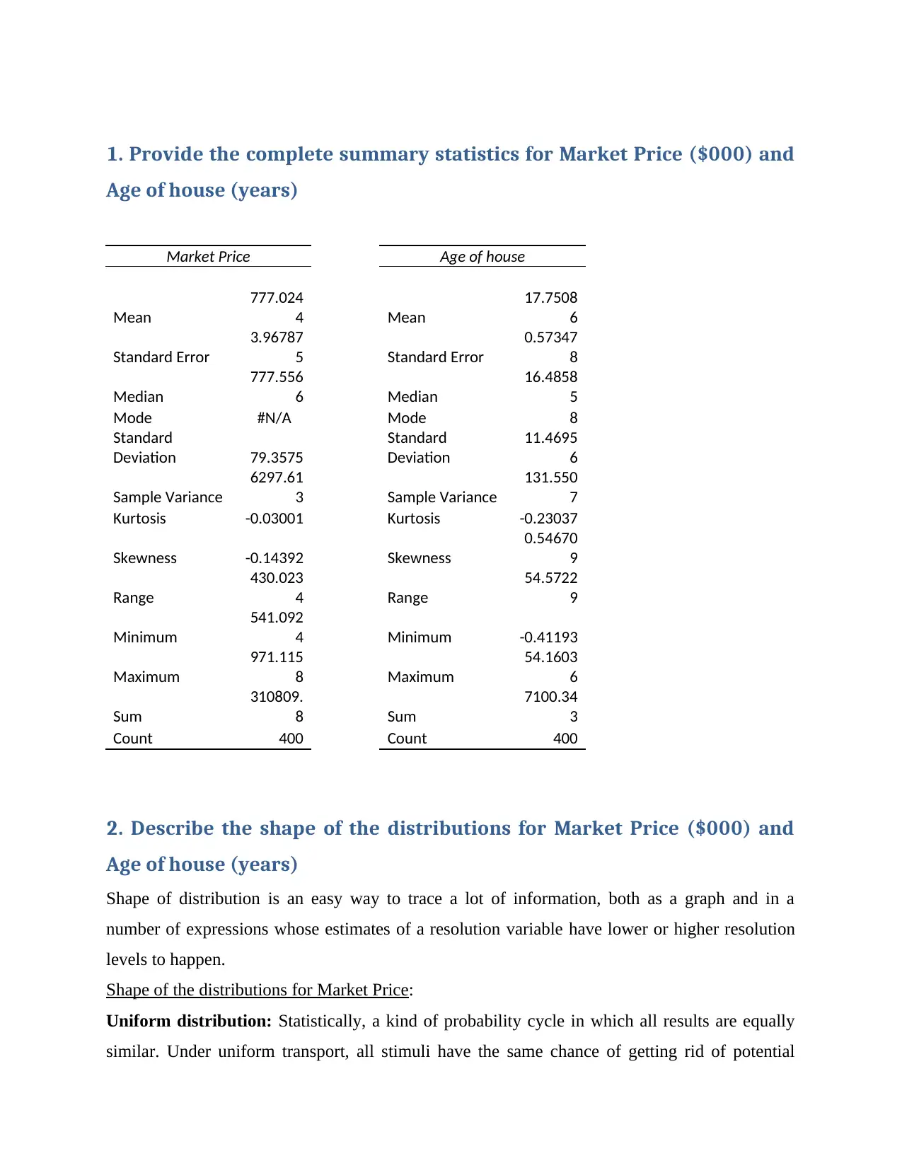
1. Provide the complete summary statistics for Market Price ($000) and
Age of house (years)
Market Price Age of house
Mean
777.024
4 Mean
17.7508
6
Standard Error
3.96787
5 Standard Error
0.57347
8
Median
777.556
6 Median
16.4858
5
Mode #N/A Mode 8
Standard
Deviation 79.3575
Standard
Deviation
11.4695
6
Sample Variance
6297.61
3 Sample Variance
131.550
7
Kurtosis -0.03001 Kurtosis -0.23037
Skewness -0.14392 Skewness
0.54670
9
Range
430.023
4 Range
54.5722
9
Minimum
541.092
4 Minimum -0.41193
Maximum
971.115
8 Maximum
54.1603
6
Sum
310809.
8 Sum
7100.34
3
Count 400 Count 400
2. Describe the shape of the distributions for Market Price ($000) and
Age of house (years)
Shape of distribution is an easy way to trace a lot of information, both as a graph and in a
number of expressions whose estimates of a resolution variable have lower or higher resolution
levels to happen.
Shape of the distributions for Market Price:
Uniform distribution: Statistically, a kind of probability cycle in which all results are equally
similar. Under uniform transport, all stimuli have the same chance of getting rid of potential
Age of house (years)
Market Price Age of house
Mean
777.024
4 Mean
17.7508
6
Standard Error
3.96787
5 Standard Error
0.57347
8
Median
777.556
6 Median
16.4858
5
Mode #N/A Mode 8
Standard
Deviation 79.3575
Standard
Deviation
11.4695
6
Sample Variance
6297.61
3 Sample Variance
131.550
7
Kurtosis -0.03001 Kurtosis -0.23037
Skewness -0.14392 Skewness
0.54670
9
Range
430.023
4 Range
54.5722
9
Minimum
541.092
4 Minimum -0.41193
Maximum
971.115
8 Maximum
54.1603
6
Sum
310809.
8 Sum
7100.34
3
Count 400 Count 400
2. Describe the shape of the distributions for Market Price ($000) and
Age of house (years)
Shape of distribution is an easy way to trace a lot of information, both as a graph and in a
number of expressions whose estimates of a resolution variable have lower or higher resolution
levels to happen.
Shape of the distributions for Market Price:
Uniform distribution: Statistically, a kind of probability cycle in which all results are equally
similar. Under uniform transport, all stimuli have the same chance of getting rid of potential
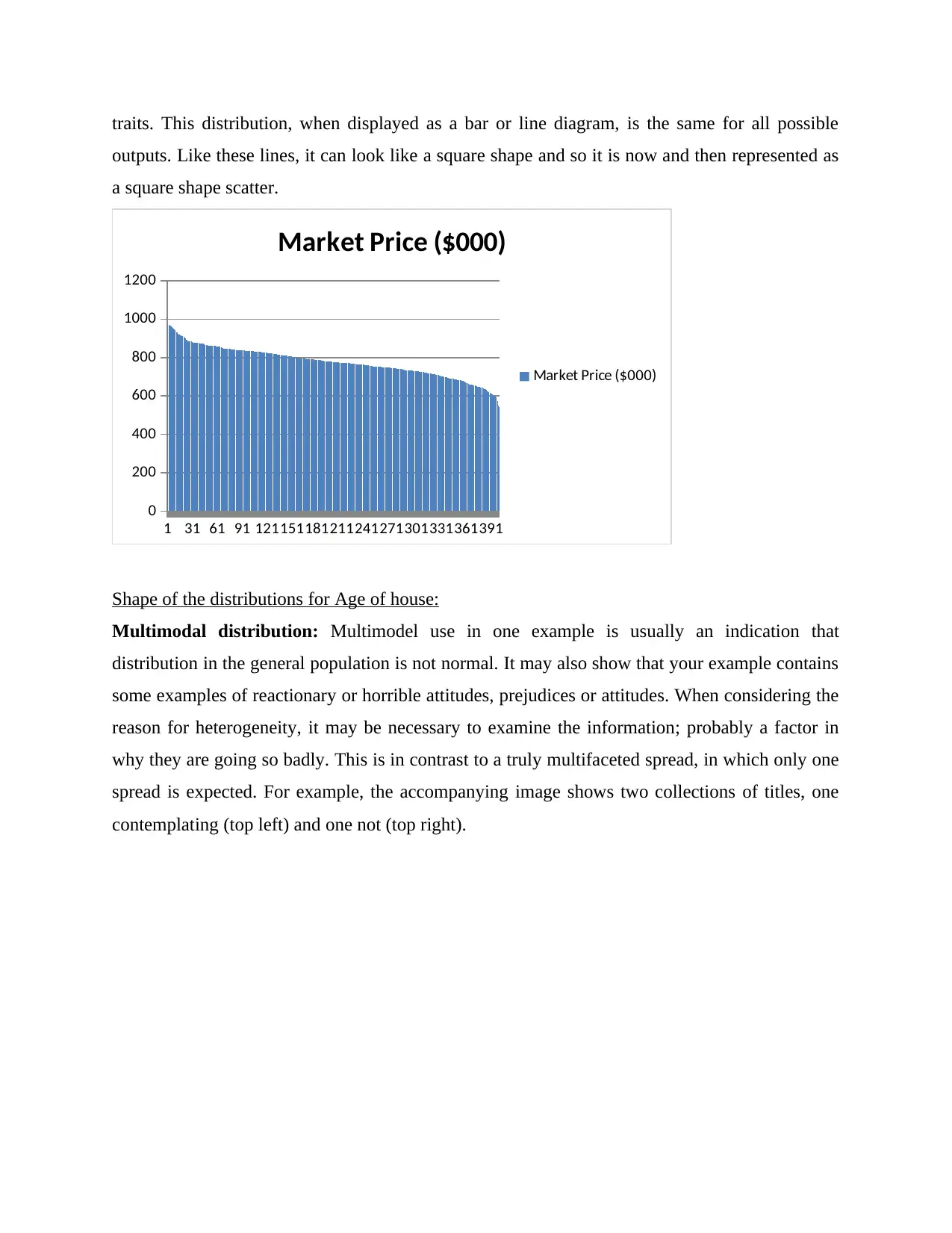
traits. This distribution, when displayed as a bar or line diagram, is the same for all possible
outputs. Like these lines, it can look like a square shape and so it is now and then represented as
a square shape scatter.
1 31 61 91 121151181211241271301331361391
0
200
400
600
800
1000
1200
Market Price ($000)
Market Price ($000)
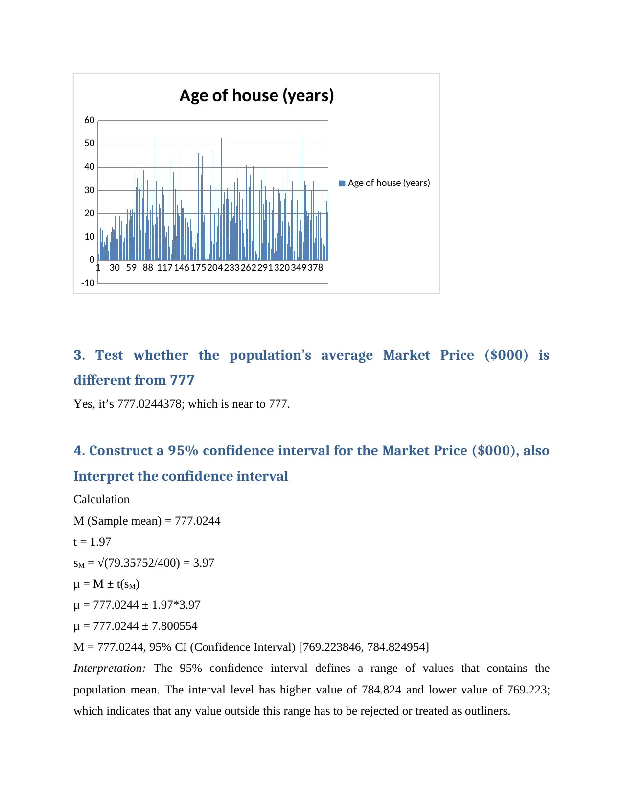
Shape of the distributions for Age of house:
Multimodal distribution: Multimodel use in one example is usually an indication that
distribution in the general population is not normal. It may also show that your example contains
some examples of reactionary or horrible attitudes, prejudices or attitudes. When considering the
reason for heterogeneity, it may be necessary to examine the information; probably a factor in
why they are going so badly. This is in contrast to a truly multifaceted spread, in which only one
spread is expected. For example, the accompanying image shows two collections of titles, one
contemplating (top left) and one not (top right).
outputs. Like these lines, it can look like a square shape and so it is now and then represented as
a square shape scatter.
1 31 61 91 121151181211241271301331361391
0
200
400
600
800
1000
1200
Market Price ($000)
Market Price ($000)
Shape of the distributions for Age of house:
Multimodal distribution: Multimodel use in one example is usually an indication that
distribution in the general population is not normal. It may also show that your example contains
some examples of reactionary or horrible attitudes, prejudices or attitudes. When considering the
reason for heterogeneity, it may be necessary to examine the information; probably a factor in
why they are going so badly. This is in contrast to a truly multifaceted spread, in which only one
spread is expected. For example, the accompanying image shows two collections of titles, one
contemplating (top left) and one not (top right).
⊘ This is a preview!⊘
Do you want full access?
Subscribe today to unlock all pages.
Trusted by 1+ million students worldwide
1 30 59 88 117 146175204233262291320349378
-10
0
10
20
30
40
50
60
Age of house (years)
Age of house (years)
3. Test whether the population’s average Market Price ($000) is
different from 777
Yes, it’s 777.0244378; which is near to 777.
4. Construct a 95% confidence interval for the Market Price ($000), also
Interpret the confidence interval
Calculation
M (Sample mean) = 777.0244
t = 1.97
sM = √(79.35752/400) = 3.97
μ = M ± t(sM)
μ = 777.0244 ± 1.97*3.97
μ = 777.0244 ± 7.800554
M = 777.0244, 95% CI (Confidence Interval) [769.223846, 784.824954]
Interpretation: The 95% confidence interval defines a range of values that contains the
population mean. The interval level has higher value of 784.824 and lower value of 769.223;
which indicates that any value outside this range has to be rejected or treated as outliners.
Paraphrase This Document
Need a fresh take? Get an instant paraphrase of this document with our AI Paraphraser
5. Provide an introduction section on the rationale of your model,
sample size, and the dependent and independent variables (including
their unit of measurement) in this model
The random sampling method makes sure that there is unbiasness in picking up of data. This
model have random data table where last two indicates row and third last digit columns; which
avoids repetition of data and its chronology. This model will show the affect of variable factors
which are dependent and independent. Some of the techniques used in this model are linear
regression, multiple regression and descriptive statistical methods.
The given data has 400 sample size in which Market price which is denoted in $000 is dependent
on independent variables which are age of the house in years and total number of square meters
in square meter. All the variables have different unit of measurement and any increasing and
decreasing in area of land and age of house impacts its prices in dollars.
6. Plot the dependent variable against each independent variable using
scatter plot/dot function in Excel. Examine these scatter plots and
correctly assess the strength and the nature of the relationship between
the dependent and the independent variables?
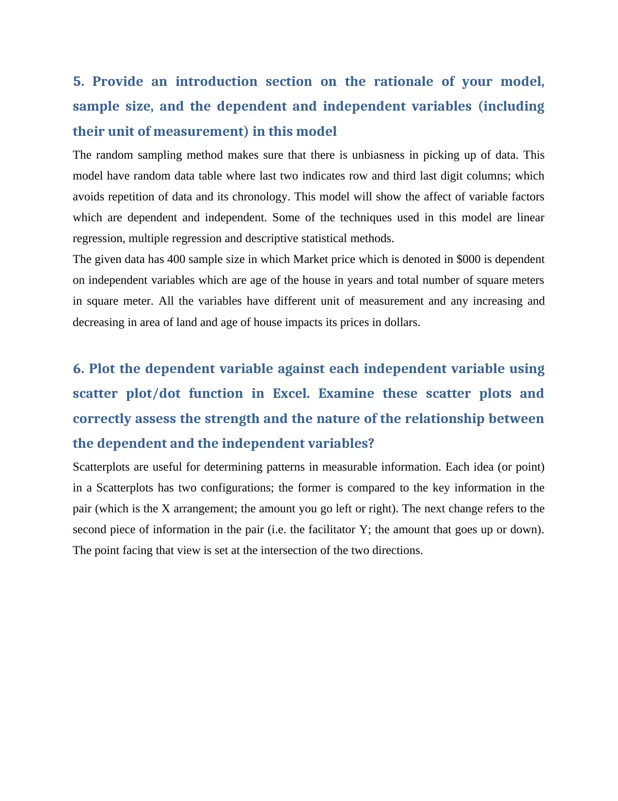
Scatterplots are useful for determining patterns in measurable information. Each idea (or point)
in a Scatterplots has two configurations; the former is compared to the key information in the
pair (which is the X arrangement; the amount you go left or right). The next change refers to the
second piece of information in the pair (i.e. the facilitator Y; the amount that goes up or down).
The point facing that view is set at the intersection of the two directions.
sample size, and the dependent and independent variables (including
their unit of measurement) in this model
The random sampling method makes sure that there is unbiasness in picking up of data. This
model have random data table where last two indicates row and third last digit columns; which
avoids repetition of data and its chronology. This model will show the affect of variable factors
which are dependent and independent. Some of the techniques used in this model are linear
regression, multiple regression and descriptive statistical methods.
The given data has 400 sample size in which Market price which is denoted in $000 is dependent
on independent variables which are age of the house in years and total number of square meters
in square meter. All the variables have different unit of measurement and any increasing and
decreasing in area of land and age of house impacts its prices in dollars.
6. Plot the dependent variable against each independent variable using
scatter plot/dot function in Excel. Examine these scatter plots and
correctly assess the strength and the nature of the relationship between
the dependent and the independent variables?
Scatterplots are useful for determining patterns in measurable information. Each idea (or point)
in a Scatterplots has two configurations; the former is compared to the key information in the
pair (which is the X arrangement; the amount you go left or right). The next change refers to the
second piece of information in the pair (i.e. the facilitator Y; the amount that goes up or down).
The point facing that view is set at the intersection of the two directions.
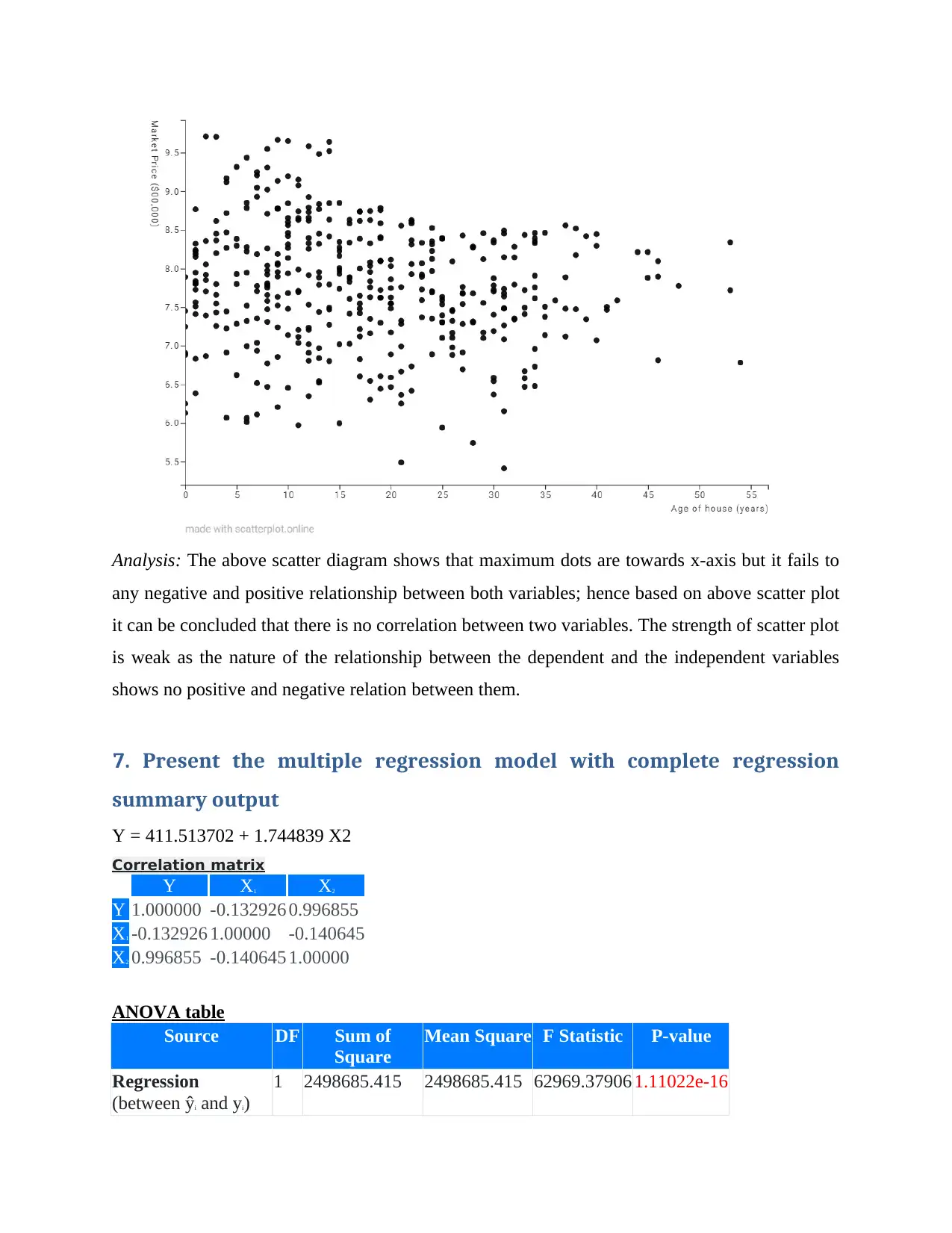
Analysis: The above scatter diagram shows that maximum dots are towards x-axis but it fails to
any negative and positive relationship between both variables; hence based on above scatter plot
it can be concluded that there is no correlation between two variables. The strength of scatter plot
is weak as the nature of the relationship between the dependent and the independent variables
shows no positive and negative relation between them.
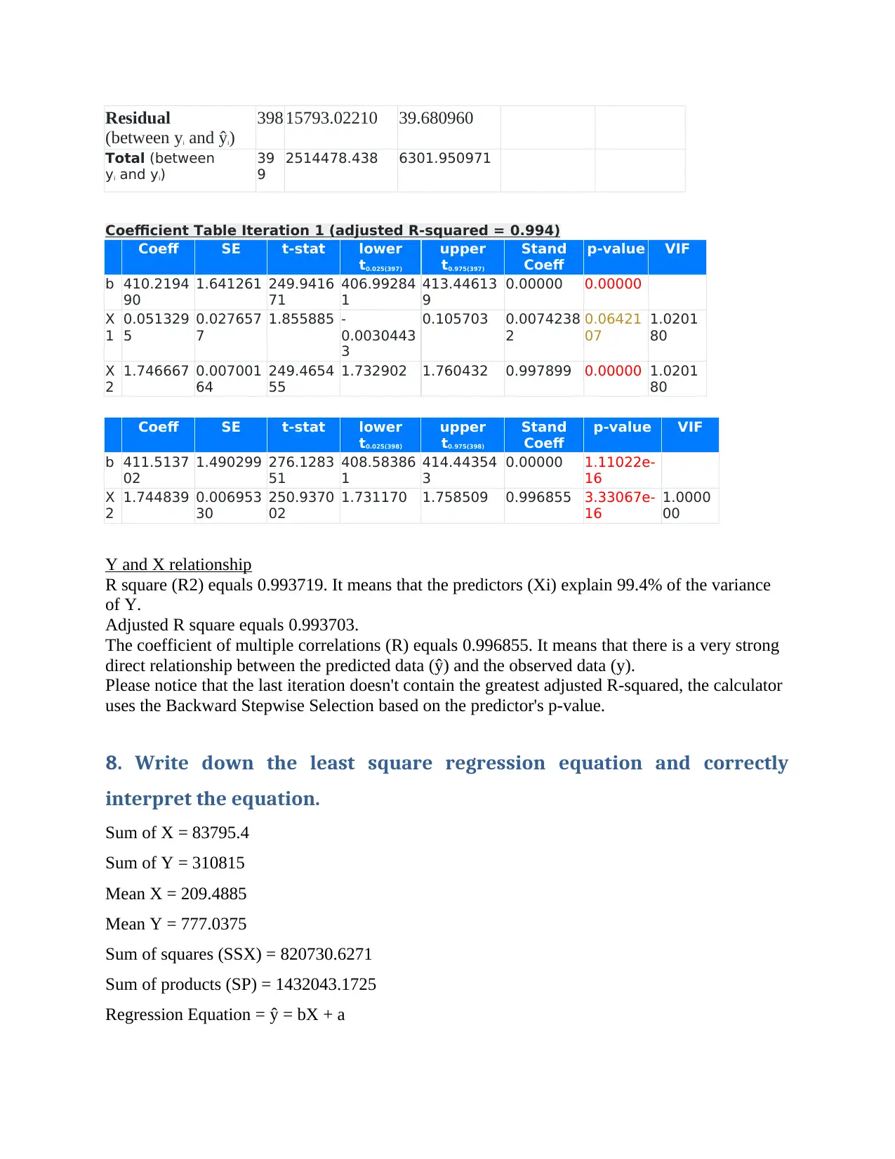
7. Present the multiple regression model with complete regression
summary output
Y = 411.513702 + 1.744839 X2
Correlation matrix
Y X1 X2
Y 1.000000 -0.132926 0.996855
X1 -0.132926 1.00000 -0.140645
X2 0.996855 -0.140645 1.00000
ANOVA table
Source DF Sum of
Square
Mean Square F Statistic P-value
Regression
(between ŷi and yi)
1 2498685.415 2498685.415 62969.37906 1.11022e-16
any negative and positive relationship between both variables; hence based on above scatter plot
it can be concluded that there is no correlation between two variables. The strength of scatter plot
is weak as the nature of the relationship between the dependent and the independent variables
shows no positive and negative relation between them.
7. Present the multiple regression model with complete regression
summary output
Y = 411.513702 + 1.744839 X2
Correlation matrix
Y X1 X2
Y 1.000000 -0.132926 0.996855
X1 -0.132926 1.00000 -0.140645
X2 0.996855 -0.140645 1.00000
ANOVA table
Source DF Sum of
Square
Mean Square F Statistic P-value
Regression
(between ŷi and yi)
1 2498685.415 2498685.415 62969.37906 1.11022e-16
⊘ This is a preview!⊘
Do you want full access?
Subscribe today to unlock all pages.
Trusted by 1+ million students worldwide
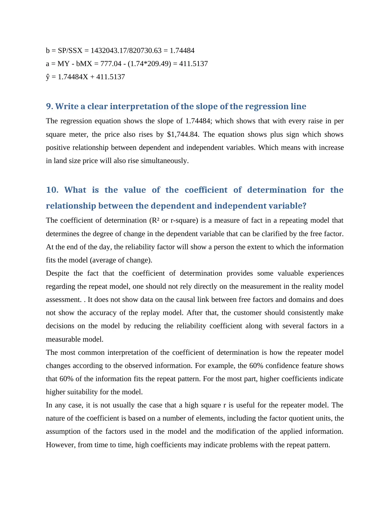
Residual
(between yi and ŷi)
398 15793.02210 39.680960
Total (between
yi and yi)
39
9
2514478.438 6301.950971
Coefficient Table Iteration 1 (adjusted R-squared = 0.994)
Coeff SE t-stat lower
t0.025(397)
upper
t0.975(397)
Stand
Coeff
p-value VIF
b 410.2194
90
1.641261 249.9416
71
406.99284
1
413.44613
9
0.00000 0.00000
X
1
0.051329
5
0.027657
7
1.855885 -
0.0030443
3
0.105703 0.0074238
2
0.06421
07
1.0201
80
X
2
1.746667 0.007001
64
249.4654
55
1.732902 1.760432 0.997899 0.00000 1.0201
80
Coeff SE t-stat lower
t0.025(398)
upper
t0.975(398)
Stand
Coeff
p-value VIF
b 411.5137
02
1.490299 276.1283
51
408.58386
1
414.44354
3
0.00000 1.11022e-
16
X
2
1.744839 0.006953
30
250.9370
02
1.731170 1.758509 0.996855 3.33067e-
16
1.0000
00
Y and X relationship
R square (R2) equals 0.993719. It means that the predictors (Xi) explain 99.4% of the variance
of Y.
Adjusted R square equals 0.993703.
The coefficient of multiple correlations (R) equals 0.996855. It means that there is a very strong
direct relationship between the predicted data (ŷ) and the observed data (y).
Please notice that the last iteration doesn't contain the greatest adjusted R-squared, the calculator
uses the Backward Stepwise Selection based on the predictor's p-value.
8. Write down the least square regression equation and correctly
interpret the equation.
Sum of X = 83795.4
Sum of Y = 310815
Mean X = 209.4885
Mean Y = 777.0375
Sum of squares (SSX) = 820730.6271
Sum of products (SP) = 1432043.1725
Regression Equation = ŷ = bX + a
Paraphrase This Document
Need a fresh take? Get an instant paraphrase of this document with our AI Paraphraser
b = SP/SSX = 1432043.17/820730.63 = 1.74484
a = MY - bMX = 777.04 - (1.74*209.49) = 411.5137
ŷ = 1.74484X + 411.5137
9. Write a clear interpretation of the slope of the regression line
The regression equation shows the slope of 1.74484; which shows that with every raise in per
square meter, the price also rises by $1,744.84. The equation shows plus sign which shows
positive relationship between dependent and independent variables. Which means with increase
in land size price will also rise simultaneously.
10. What is the value of the coefficient of determination for the
relationship between the dependent and independent variable?
The coefficient of determination (R² or r-square) is a measure of fact in a repeating model that
determines the degree of change in the dependent variable that can be clarified by the free factor.
At the end of the day, the reliability factor will show a person the extent to which the information
fits the model (average of change).
Despite the fact that the coefficient of determination provides some valuable experiences
regarding the repeat model, one should not rely directly on the measurement in the reality model
assessment. . It does not show data on the causal link between free factors and domains and does
not show the accuracy of the replay model. After that, the customer should consistently make
decisions on the model by reducing the reliability coefficient along with several factors in a
measurable model.
The most common interpretation of the coefficient of determination is how the repeater model
changes according to the observed information. For example, the 60% confidence feature shows
that 60% of the information fits the repeat pattern. For the most part, higher coefficients indicate
higher suitability for the model.
In any case, it is not usually the case that a high square r is useful for the repeater model. The
nature of the coefficient is based on a number of elements, including the factor quotient units, the
assumption of the factors used in the model and the modification of the applied information.
However, from time to time, high coefficients may indicate problems with the repeat pattern.
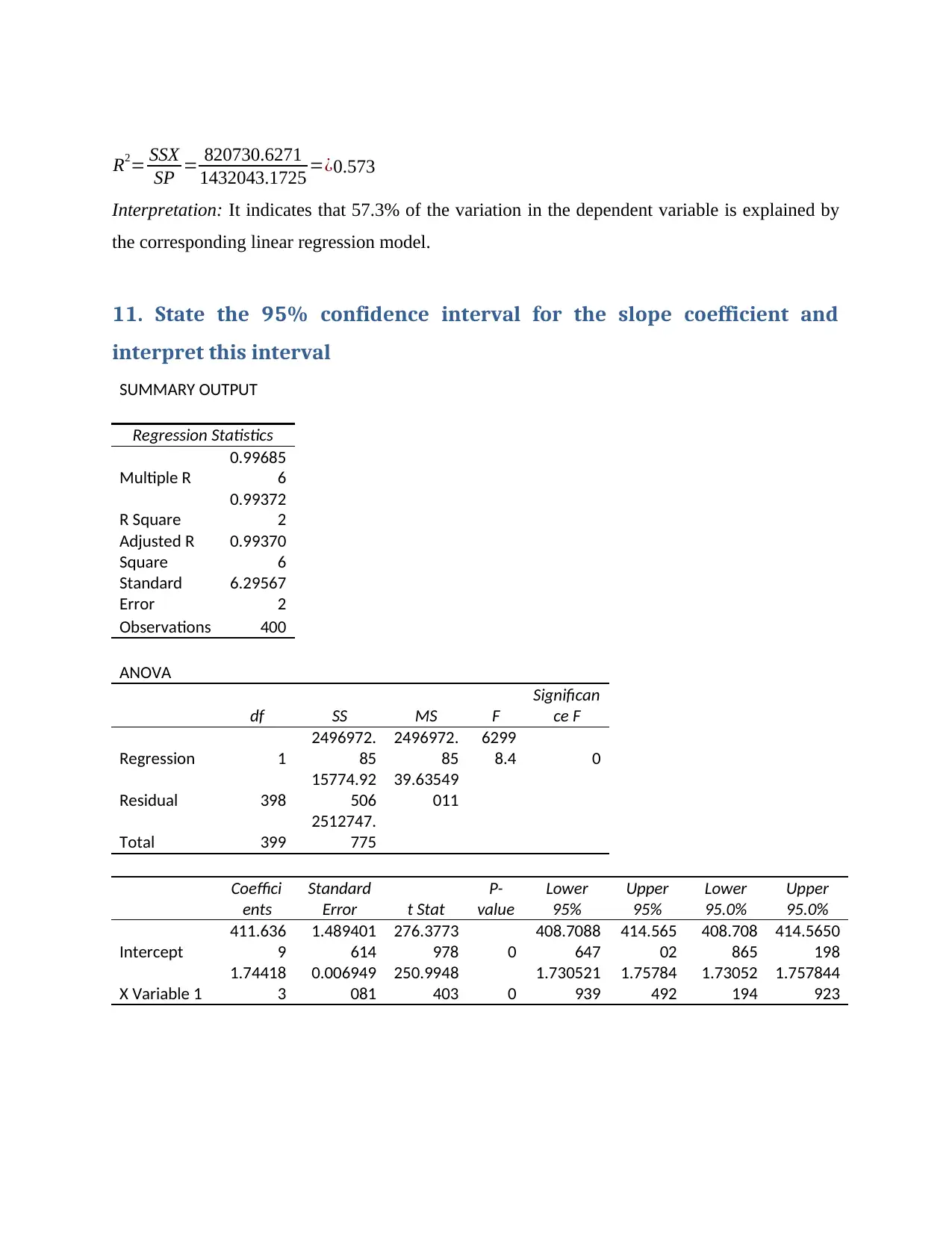
R2= SSX
SP = 820730.6271
1432043.1725 =¿0.573
Interpretation: It indicates that 57.3% of the variation in the dependent variable is explained by
the corresponding linear regression model.
11. State the 95% confidence interval for the slope coefficient and
interpret this interval
SUMMARY OUTPUT
Regression Statistics
Multiple R
0.99685
6
R Square
0.99372
2
Adjusted R
Square
0.99370
6
Standard
Error
6.29567
2
Observations 400
ANOVA
df SS MS F
Significan
ce F
Regression 1
2496972.
85
2496972.
85
6299
8.4 0
Residual 398
15774.92
506
39.63549
011
Total 399
2512747.
775
Coeffici
ents
Standard
Error t Stat
P-
value
Lower
95%
Upper
95%
Lower
95.0%
Upper
95.0%
Intercept
411.636
9
1.489401
614
276.3773
978 0
408.7088
647
414.565
02
408.708
865
414.5650
198
X Variable 1
1.74418
3
0.006949
081
250.9948
403 0
1.730521
939
1.75784
492
1.73052
194
1.757844
923
⊘ This is a preview!⊘
Do you want full access?
Subscribe today to unlock all pages.
Trusted by 1+ million students worldwide
Interpretation: In previous case the slope was at 1.74484 but at 95% confidence level the slope
has been declined to 1.744183; on the other hand the intercept value has increased from
411.5137 to 411.6369.
12. Compare the multiple regression models (question 7) and simple
linear regression model (question 8) and evaluate the goodness of fit
between these two modeling techniques
Regression analysis is a standard way of measuring the value of an asset and contributing to it.
Linear regression is just one of the best known strategies for repeating the analysis. Multiple
regression are a larger class of repetitions that include direct and unrelated repetitions with a
number of information factors.
Regression as a tool causes the collection of information to help people and organizations decide
educational choices. There are a number of factors that influence everything in a repeater,
including a required variable - the base variable you are trying to understand - and an
autonomous variable - factors that could influence the reliable variable.
Linear Regression
Also known as simple linear regression. Build the connection between two factors using a
straight line. The repetitions simply try to draw a line closer to the information by finding the
slant and capturing that marks the line and limits playback errors.
Multiple Regressions
It is rare that a variable needs to be clarified by a single variable. For this scenario, an analyst
uses a series of repetitions, which try to clarify a required variable by using more than one free
factor. Multiple repetitions can be direct and unrelated.
Multiple Regression are based on the suspicion that there is a direct link between dependent and
autonomous factors. It is also expected that there will be no significant relationship between the
free factors.
Goodness of fit
Overall regression: right-tailed, F (1,398) = 62969.37906, p-value = 1.11022e-16. Since p-value
< α (0.05), we reject the H0.
The linear regression model, Y = b0+ b1X1 +...+bpXp, provides a better fit than the model
without the independent variables resulting in, Y = b0.
The following independent variable is not significant as predictors for Y: X1.
Therefore it was excluded from the model.
Paraphrase This Document
Need a fresh take? Get an instant paraphrase of this document with our AI Paraphraser
If any excluded variable is highly suspected to be related to the dependent variable (Y),
theoretically or due to previous research, it is recommended to include the variable in the model
irrespective of the p-value, to do it, you should change the iterations to manual.
The Y-intercept (b): two-tailed, T = 276.128351, p-value = 1.11022e-16. Hence b is significantly
different from zero.
13. Predict the market price of a house (in $) with a building area of 300
square meters
ŷ = 1.74484X + 411.5137
ŷ = 1.74484 (300) + 411.5137
ŷ = 934.9657 or $934,965.7
14 & 15. Statistical analysis involving hypothesis testing
The basic issue is to find whether the Land size in Square meters useful in predicting the
market price of a house (in $). To answer this question two hypotheses can be made; null and
alternate hypothesis. In this case to test whether the model is complete useless or not; F-test is
best fit to know the answer. For this purpose the hypotheses statement will support in find out the
conclusion:
Null hypotheses H0 = Not useful for prediction
Alternate hypothesis H1 = Useful for prediction.
The significant value of α = 0.95 or 95% confidence level
Coefficients
Standard
Error t Stat P-value
Intercept
411.63694
2 1.489401614
276.3
8 0
Total number of square meters
1.7441834
3 0.006949081
250.9
9 0
Conclusion: Here; p value of predictor variable which is total number of square meters is
statistically significant as it is less than alpha value which is 0.05. Hence; null hypothesis will be
rejected and alternate hypothesis will be accepted and it can be concluded that the above variable
and tools are useful in predicting the market price of house in $.
1 out of 11
Related Documents


Your All-in-One AI-Powered Toolkit for Academic Success.
+13062052269
info@desklib.com
Available 24*7 on WhatsApp / Email
![[object Object]](/_next/static/media/star-bottom.7253800d.svg)
Unlock your academic potential
Copyright © 2020–2026 A2Z Services. All Rights Reserved. Developed and managed by ZUCOL.