Statistics Homework: Frequency Distribution, Regression, and Analysis

This statistics assignment presents solutions to a variety of statistical problems. Question 1 focuses on preparing frequency, relative, and percent frequency distributions, along with constructing a histogram. Question 2 delves into regression analysis, including developing a regression equation, determining the coefficient of determination (R2), and interpreting the relationship between variables. Question 3 assesses sample sizes for different treatments, and Question 4 involves developing and interpreting a multiple regression equation, identifying relationships between variables, and assessing the significance of regression coefficients. The solutions provide detailed calculations, interpretations, and statistical tests to address each problem.

Statics Question

TABLE OF CONTENTS
QUESTION 1..................................................................................................................................3
a. Prepare a frequency, relative and percent frequency distribution for the data set using a class
width of $50.................................................................................................................................3
b. Construct a histogram showing the percent frequency distribution of the furnitureorder
values...........................................................................................................................................3
c....................................................................................................................................................4
QUESTION 2..................................................................................................................................4
a....................................................................................................................................................4
b...................................................................................................................................................5
c....................................................................................................................................................5
QUESTION 3..................................................................................................................................5
Assessing whether sample sizes for the three treatments are equal.............................................5
QUESTION 4..................................................................................................................................6
a. Developing an estimate regression equatuion related to y to X1 & X2...................................6
b. identifying relationship betweem dependent and independent variables...............................6
c. Assessing whether β1 and β2 is different from zero...............................................................6
d. Interpreting slope co-efficient for X2......................................................................................8
e. Assessing the number of mobile phones which one expect to sell in a day............................8

QUESTION 1
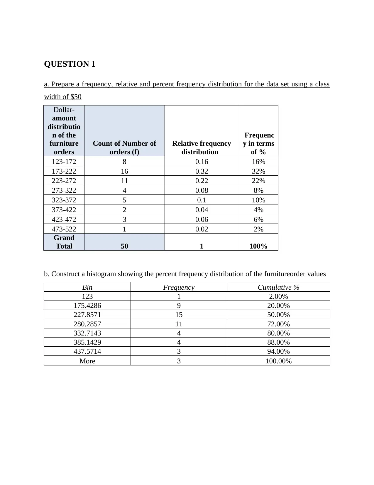
a. Prepare a frequency, relative and percent frequency distribution for the data set using a class
width of $50
Dollar-
amount
distributio
n of the
furniture
orders
Count of Number of
orders (f)
Relative frequency
distribution
Frequenc
y in terms
of %
123-172 8 0.16 16%
173-222 16 0.32 32%
223-272 11 0.22 22%
273-322 4 0.08 8%
323-372 5 0.1 10%
373-422 2 0.04 4%
423-472 3 0.06 6%
473-522 1 0.02 2%
Grand
Total 50 1 100%
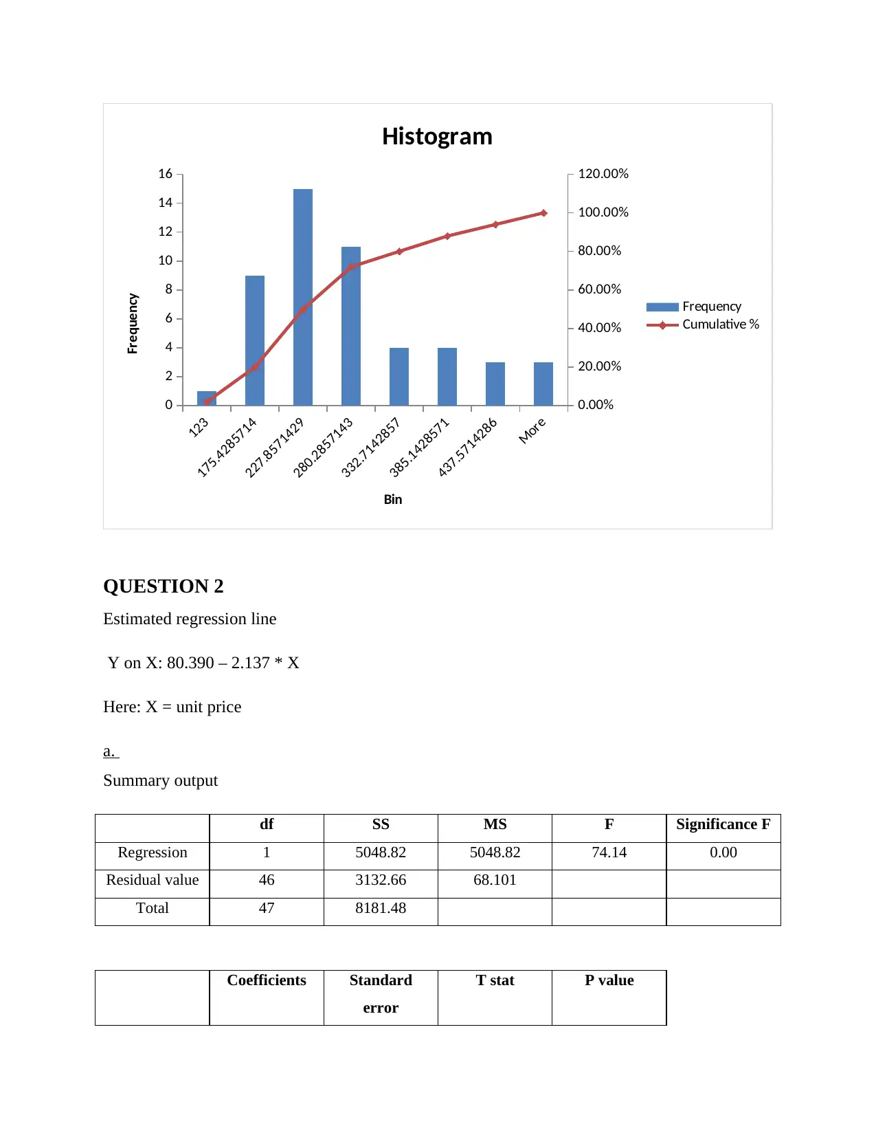
b. Construct a histogram showing the percent frequency distribution of the furnitureorder values
Bin Frequency Cumulative %
123 1 2.00%
175.4286 9 20.00%
227.8571 15 50.00%
280.2857 11 72.00%
332.7143 4 80.00%
385.1429 4 88.00%
437.5714 3 94.00%
More 3 100.00%

123
175.4285714
227.8571429
280.2857143
332.7142857
385.1428571
437.5714286
More
0
2
4
6
8
10
12
14
16
0.00%
20.00%
40.00%
60.00%
80.00%
100.00%
120.00%
Histogram
Frequency
Cumulative %
Bin
Frequency
QUESTION 2
Estimated regression line
Y on X: 80.390 – 2.137 * X
Here: X = unit price
a.
Summary output
df SS MS F Significance F
Regression 1 5048.82 5048.82 74.14 0.00
Residual value 46 3132.66 68.101
Total 47 8181.48
Coefficients Standard
error
T stat P value

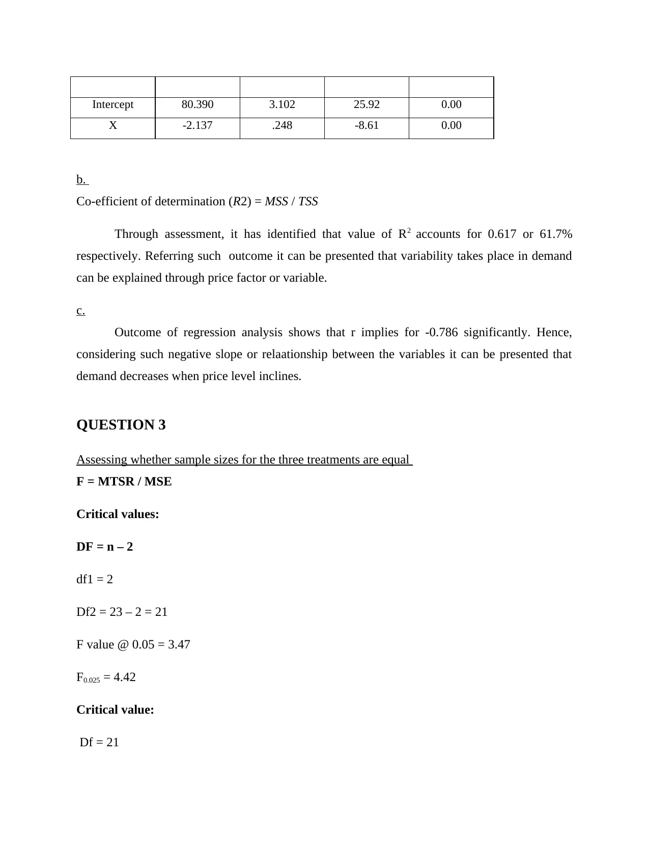
Intercept 80.390 3.102 25.92 0.00
X -2.137 .248 -8.61 0.00
b.
Co-efficient of determination (R2) = MSS / TSS
Through assessment, it has identified that value of R2 accounts for 0.617 or 61.7%
respectively. Referring such outcome it can be presented that variability takes place in demand
can be explained through price factor or variable.
c.
Outcome of regression analysis shows that r implies for -0.786 significantly. Hence,
considering such negative slope or relaationship between the variables it can be presented that
demand decreases when price level inclines.
QUESTION 3
Assessing whether sample sizes for the three treatments are equal
F = MTSR / MSE
Critical values:
DF = n – 2
df1 = 2
Df2 = 23 – 2 = 21
F value @ 0.05 = 3.47
F0.025 = 4.42
Critical value:
Df = 21

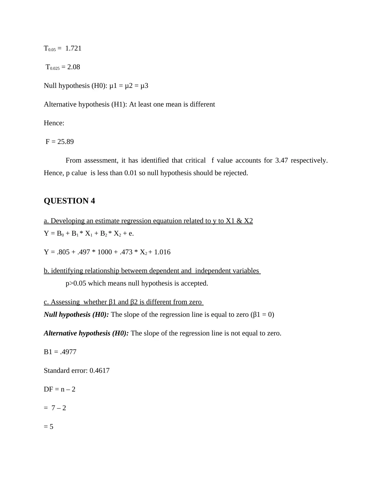
T0.05 = 1.721
T0.025 = 2.08
Null hypothesis (H0): μ1 = μ2 = μ3
Alternative hypothesis (H1): At least one mean is different
Hence:
F = 25.89
From assessment, it has identified that critical f value accounts for 3.47 respectively.
Hence, p calue is less than 0.01 so null hypothesis should be rejected.
QUESTION 4
a. Developing an estimate regression equatuion related to y to X1 & X2
Y = B0 + B1 * X1 + B2 * X2 + e.
Y = .805 + .497 * 1000 + .473 * X2 + 1.016
b. identifying relationship betweem dependent and independent variables
p>0.05 which means null hypothesis is accepted.
c. Assessing whether β1 and β2 is different from zero
Null hypothesis (H0): The slope of the regression line is equal to zero (β1 = 0)
Alternative hypothesis (H0): The slope of the regression line is not equal to zero.
Β1 = .4977
Standard error: 0.4617
DF = n – 2
= 7 – 2
= 5

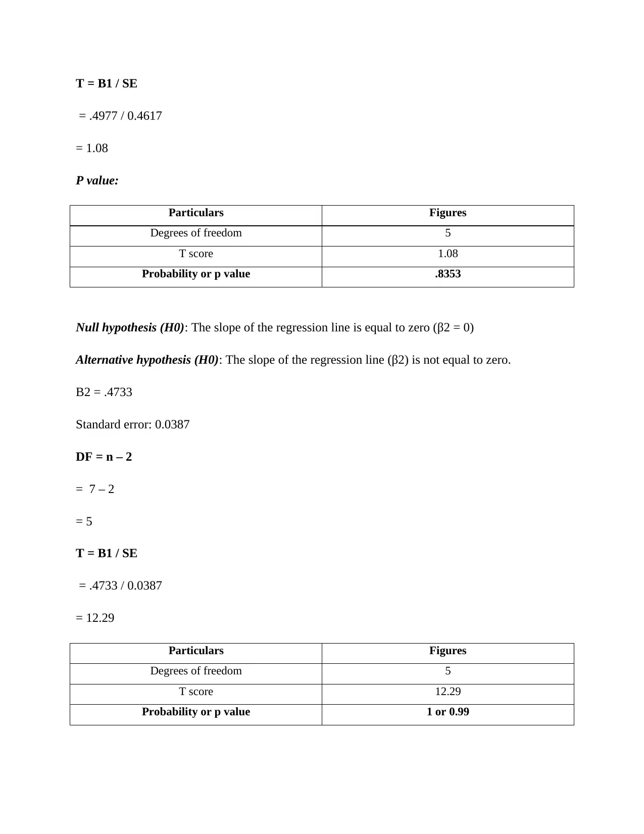
T = B1 / SE
= .4977 / 0.4617
= 1.08
P value:
Particulars Figures
Degrees of freedom 5
T score 1.08
Probability or p value .8353
Null hypothesis (H0): The slope of the regression line is equal to zero (β2 = 0)
Alternative hypothesis (H0): The slope of the regression line (β2) is not equal to zero.
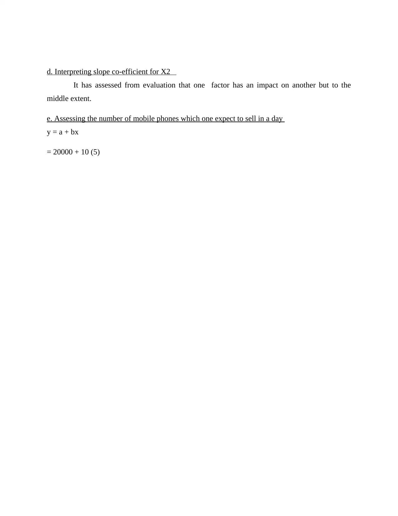
Β2 = .4733
Standard error: 0.0387
DF = n – 2
= 7 – 2
= 5
T = B1 / SE
= .4733 / 0.0387
= 12.29
Particulars Figures
Degrees of freedom 5
T score 12.29
Probability or p value 1 or 0.99

d. Interpreting slope co-efficient for X2
It has assessed from evaluation that one factor has an impact on another but to the
middle extent.
e. Assessing the number of mobile phones which one expect to sell in a day
y = a + bx
= 20000 + 10 (5)