Holmes Institute HI6007 Statistics Group Assignment: Data Analysis

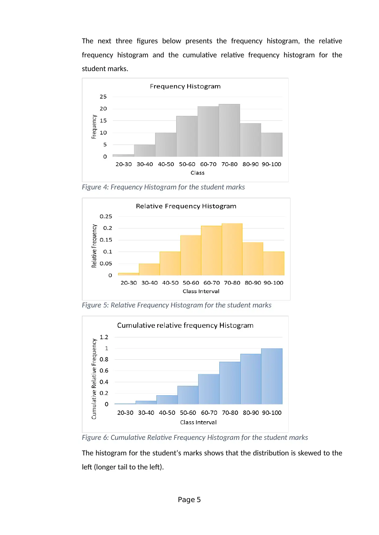
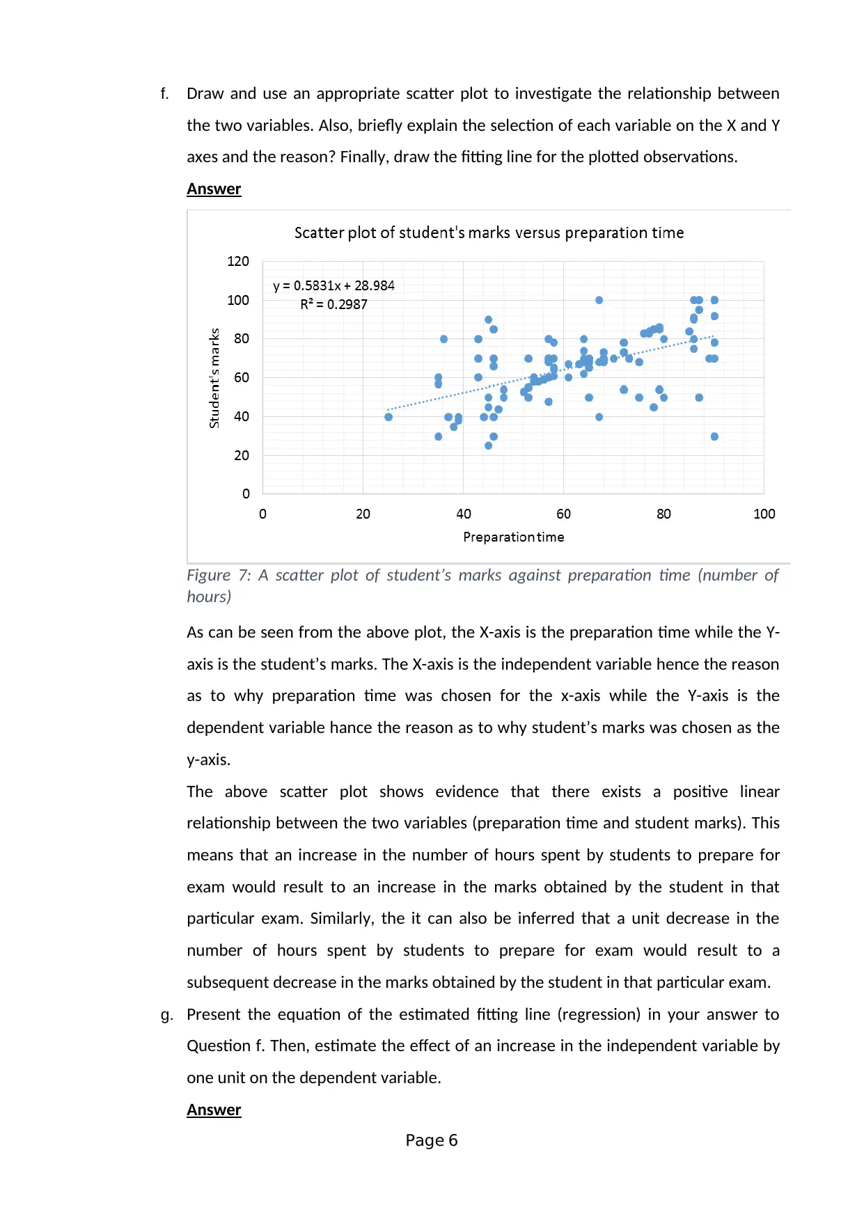
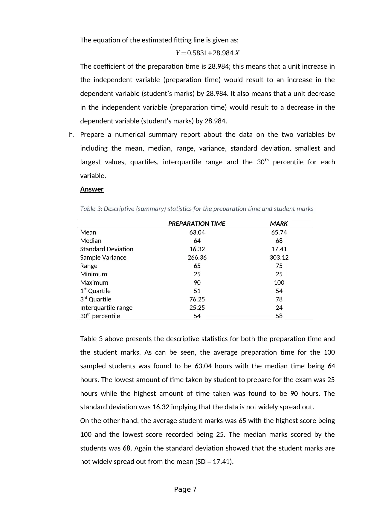
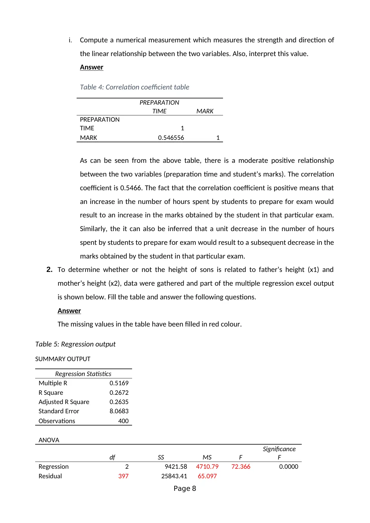
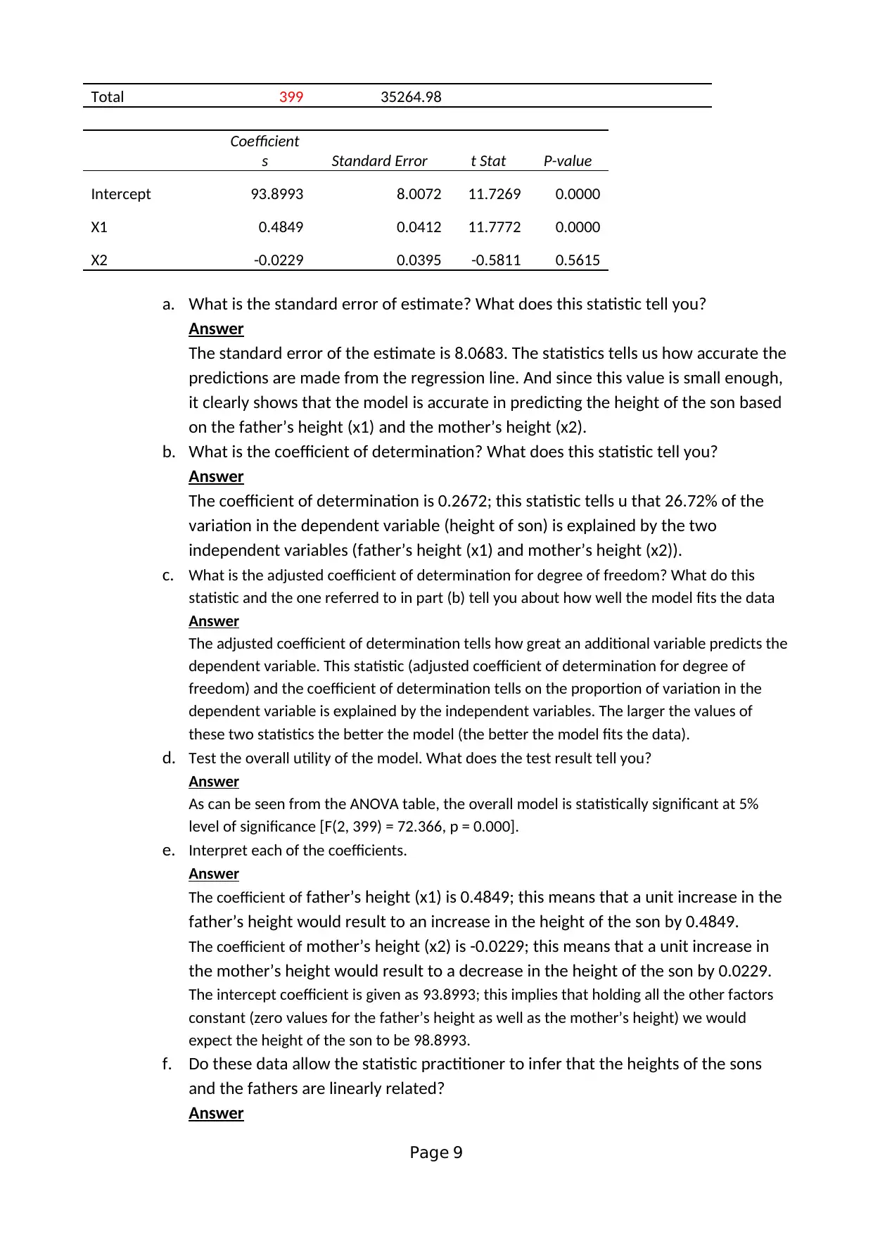
This assignment solution addresses a statistics group assignment (HI6007) from Holmes Institute, focusing on analyzing the relationship between students' preparation time for an exam and their marks. The solution employs a cross-sectional survey method and simple random sampling to collect data from 100 students. It identifies dependent and independent variables, discusses potential data collection issues, and develops frequency distributions with histograms to visualize data patterns. The assignment utilizes scatter plots and regression analysis to investigate the relationship between variables, providing the regression equation and interpreting coefficients. Furthermore, it presents a descriptive statistical summary, including mean, median, standard deviation, and correlation coefficients. The second part of the assignment involves multiple regression analysis, interpreting the output to determine relationships between son's height and parents' heights, including the standard error, coefficient of determination, and model utility.

HOLMES INSTITUTE
FACULTY OF HIGHER EDUCATION
HI6007 Group Assignment
Due End of Week/Lecture 10
WORTH 30%
Please read below information carefully and respond all questions listed.
Page 1

1. Many Holmes Institute instructors believe that students need to spend at least 2 hours
studying outside of class for every hour of lecture. They believe that the number of hours
students study to prepare for the exam affect students’ marks significantly. As opposed,
few of the lecturers believe that the number of preparation hours do not essentially affect
students’ marks while some other factors are to be considered. To study the relationship
between the preparation time spent by each student (in hours) for the exam and the
reported mark, a sample of 100 students were selected randomly from a large statistics
class. The data are stored in the file named “ASSIGNMENTDATA” in the course website.
Answer below 9 questions:
a. What type of survey method could be used? Explain your answer.
Answer
Cross-sectional survey; this is where the researcher collects data from the
respondents at a single period in time uses the cross-sectional type of survey.
b. What sampling method could be used to select the sample? Explain your answer.
Answer
Simple random sampling could be used. This method would give the participants an
equal chance of being included into the study and as such will reduce the chances
of bias.
c. On the basis of given data, determine the dependent and independent variables we
should use, and why? Also, identify the data type(s) for each variable.
Answer
The dependent variable is the student’s marks while the independent variable is the
number of hours students study to prepare for the exam. This is because number of
hours students study to prepare for the exam is believed to influence the students
marks hence it is the independent variable while the student marks is the
dependent variable.
d. What kind of issues we may face in collecting the data using this type of survey
method? List and explain two cases.
Answer
Some of the issues that might be faced include;
 Non-response from some of the participants. Some participants might not
be willing to respond for their own reasons.
Page 2

 High cost of collecting data; one challenge would be in regard to the cost if
the participants are widely spread apart.
e. Using 8 classes and intervals of 20 - 30, 30 - 40, etc for both of the variables
selected in question 3, develop a distribution table including class intervals,
frequency, relative frequency and cumulative relative frequency for each variable.
Then, draw frequency histogram, relative frequency histogram and cumulative
relative frequency histogram for each variable. Also, Comment on the shape of
frequency histogram for each variable and provide reason(s) for your comment.
Answer
Table 1 Distribution table for preparation time
Class
Interval
Frequency Relative
Frequency
Cumulative relative
frequency
20-30 1 0.01 0.01
30-40 8 0.08 0.09
40-50 16 0.16 0.25
50-60 20 0.2 0.45
60-70 20 0.2 0.65
70-80 17 0.17 0.82
80-90 12 0.12 0.94
90-100 6 0.06 1
Table 2: Distribution table for student marks
Class
Interval
Frequency Relative
Frequency
Cumulative relative
frequency
20-30 1 0.01 0.01
30-40 5 0.05 0.06
40-50 10 0.1 0.16
50-60 17 0.17 0.33
60-70 21 0.21 0.54
70-80 22 0.22 0.76
80-90 14 0.14 0.9
90-100 10 0.1 1
Histograms for the preparation time
Page 3

In the next three figures, we present the frequency histogram, the relative
frequency histogram and the cumulative relative frequency histogram for the
preparation time. The histogram help to visualize the distribution of the data.
Figure 1: Frequency Histogram for the preparation time
Figure 2: Relative Frequency Histogram for the preparation time
Figure 3: Cumulative Relative Frequency Histogram for the preparation time
The histogram (both frequency and relative frequency) of the preparation time
shows that the distribution is left skewed (has longer tail to the left).
Histograms for the Student marks
Page 4

The next three figures below presents the frequency histogram, the relative
frequency histogram and the cumulative relative frequency histogram for the
student marks.
Figure 4: Frequency Histogram for the student marks
Figure 5: Relative Frequency Histogram for the student marks
Figure 6: Cumulative Relative Frequency Histogram for the student marks
The histogram for the student’s marks shows that the distribution is skewed to the
left (longer tail to the left).
Page 5

f. Draw and use an appropriate scatter plot to investigate the relationship between
the two variables. Also, briefly explain the selection of each variable on the X and Y
axes and the reason? Finally, draw the fitting line for the plotted observations.
Answer
Figure 7: A scatter plot of student’s marks against preparation time (number of
hours)
As can be seen from the above plot, the X-axis is the preparation time while the Y-
axis is the student’s marks. The X-axis is the independent variable hence the reason
as to why preparation time was chosen for the x-axis while the Y-axis is the
dependent variable hance the reason as to why student’s marks was chosen as the
y-axis.
The above scatter plot shows evidence that there exists a positive linear
relationship between the two variables (preparation time and student marks). This
means that an increase in the number of hours spent by students to prepare for
exam would result to an increase in the marks obtained by the student in that
particular exam. Similarly, the it can also be inferred that a unit decrease in the
number of hours spent by students to prepare for exam would result to a
subsequent decrease in the marks obtained by the student in that particular exam.
g. Present the equation of the estimated fitting line (regression) in your answer to
Question f. Then, estimate the effect of an increase in the independent variable by
one unit on the dependent variable.
Answer
Page 6

The equation of the estimated fitting line is given as;
Y =0.5831+28.984 X
The coefficient of the preparation time is 28.984; this means that a unit increase in
the independent variable (preparation time) would result to an increase in the
dependent variable (student’s marks) by 28.984. It also means that a unit decrease
in the independent variable (preparation time) would result to a decrease in the
dependent variable (student’s marks) by 28.984.
h. Prepare a numerical summary report about the data on the two variables by
including the mean, median, range, variance, standard deviation, smallest and
largest values, quartiles, interquartile range and the 30th percentile for each
variable.
Answer
Table 3: Descriptive (summary) statistics for the preparation time and student marks
PREPARATION TIME MARK
Mean 63.04 65.74
Median 64 68
Standard Deviation 16.32 17.41
Sample Variance 266.36 303.12
Range 65 75
Minimum 25 25
Maximum 90 100
1st Quartile 51 54
3rd Quartile 76.25 78
Interquartile range 25.25 24
30th percentile 54 58
Table 3 above presents the descriptive statistics for both the preparation time and
the student marks. As can be seen, the average preparation time for the 100
sampled students was found to be 63.04 hours with the median time being 64
hours. The lowest amount of time taken by student to prepare for the exam was 25
hours while the highest amount of time taken was found to be 90 hours. The
standard deviation was 16.32 implying that the data is not widely spread out.
On the other hand, the average student marks was 65 with the highest score being
100 and the lowest score recorded being 25. The median marks scored by the
students was 68. Again the standard deviation showed that the student marks are
not widely spread out from the mean (SD = 17.41).
Page 7

i. Compute a numerical measurement which measures the strength and direction of
the linear relationship between the two variables. Also, interpret this value.
Answer
Table 4: Correlation coefficient table
PREPARATION
TIME MARK
PREPARATION
TIME 1
MARK 0.546556 1
As can be seen from the above table, there is a moderate positive relationship
between the two variables (preparation time and student’s marks). The correlation
coefficient is 0.5466. The fact that the correlation coefficient is positive means that
an increase in the number of hours spent by students to prepare for exam would
result to an increase in the marks obtained by the student in that particular exam.
Similarly, the it can also be inferred that a unit decrease in the number of hours
spent by students to prepare for exam would result to a subsequent decrease in the
marks obtained by the student in that particular exam.
2. To determine whether or not the height of sons is related to father’s height (x1) and
mother’s height (x2), data were gathered and part of the multiple regression excel output
is shown below. Fill the table and answer the following questions.
Answer
The missing values in the table have been filled in red colour.
Table 5: Regression output
SUMMARY OUTPUT
Regression Statistics
Multiple R 0.5169
R Square 0.2672
Adjusted R Square 0.2635
Standard Error 8.0683
Observations 400
ANOVA
df SS MS F
Significance
F
Regression 2 9421.58 4710.79 72.366 0.0000
Residual 397 25843.41 65.097
Page 8

Total 399 35264.98
Coefficient
s Standard Error t Stat P-value
Intercept 93.8993 8.0072 11.7269 0.0000
X1 0.4849 0.0412 11.7772 0.0000
X2 -0.0229 0.0395 -0.5811 0.5615
a. What is the standard error of estimate? What does this statistic tell you?
Answer
The standard error of the estimate is 8.0683. The statistics tells us how accurate the
predictions are made from the regression line. And since this value is small enough,
it clearly shows that the model is accurate in predicting the height of the son based
on the father’s height (x1) and the mother’s height (x2).
b. What is the coefficient of determination? What does this statistic tell you?
Answer
The coefficient of determination is 0.2672; this statistic tells u that 26.72% of the
variation in the dependent variable (height of son) is explained by the two
independent variables (father’s height (x1) and mother’s height (x2)).
c. What is the adjusted coefficient of determination for degree of freedom? What do this
statistic and the one referred to in part (b) tell you about how well the model fits the data
Answer
The adjusted coefficient of determination tells how great an additional variable predicts the
dependent variable. This statistic (adjusted coefficient of determination for degree of
freedom) and the coefficient of determination tells on the proportion of variation in the
dependent variable is explained by the independent variables. The larger the values of
these two statistics the better the model (the better the model fits the data).
d. Test the overall utility of the model. What does the test result tell you?
Answer
As can be seen from the ANOVA table, the overall model is statistically significant at 5%
level of significance [F(2, 399) = 72.366, p = 0.000].
e. Interpret each of the coefficients.
Answer
The coefficient of father’s height (x1) is 0.4849; this means that a unit increase in the
father’s height would result to an increase in the height of the son by 0.4849.
The coefficient of mother’s height (x2) is -0.0229; this means that a unit increase in
the mother’s height would result to a decrease in the height of the son by 0.0229.
The intercept coefficient is given as 93.8993; this implies that holding all the other factors
constant (zero values for the father’s height as well as the mother’s height) we would
expect the height of the son to be 98.8993.
f. Do these data allow the statistic practitioner to infer that the heights of the sons
and the fathers are linearly related?
Answer
Page 9

Yes the data allow the statistic practitioner to infer that the heights of the sons and
the fathers are linearly related. This is based on the fact that the father’s height (x1)
was found to be significant in the model (p = 0.0000).
g. Do these data allow the statistic practitioner to infer that the heights of the sons
and the mothers are linearly related?
Answer
No the data does not allow the statistic practitioner to infer that the heights of the
sons and the mothers are linearly related. This is based on the fact that the
mother’s height (x2) was found to be insignificant in the model (p = 0.5615).
END OF THE ASSIGNMENT
Page 10