Holmes Institute HI6007 Statistics Group Assignment Solution

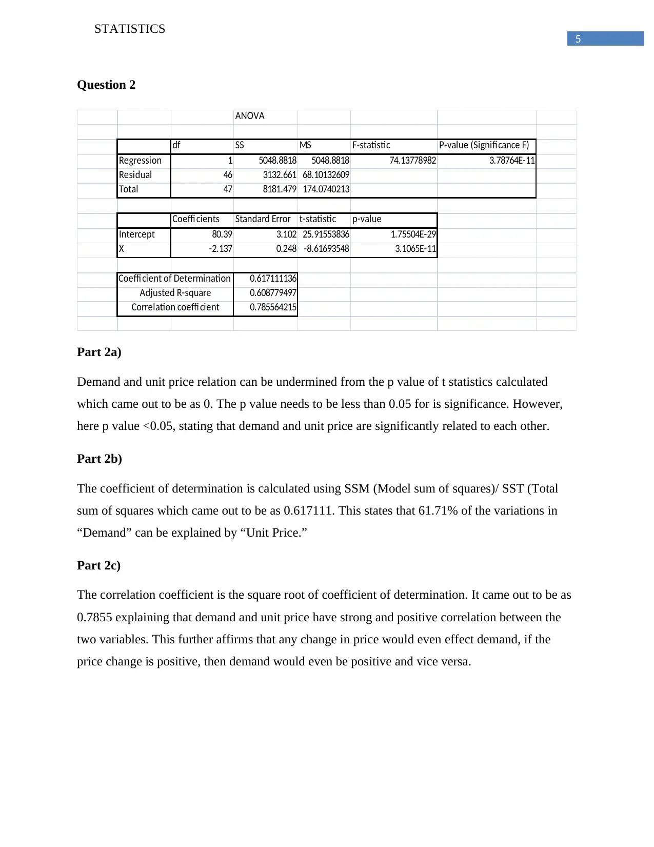
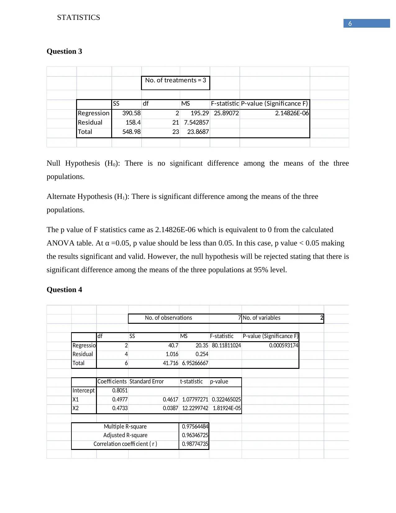
This document presents a comprehensive solution to a statistics group assignment (HI6007), covering various statistical concepts and techniques. The assignment includes an analysis of frequency distributions, including the calculation of relative frequency, percentage frequency, and the construction of a histogram. Furthermore, the solution explores regression analysis, examining the relationship between demand and unit price, calculating the coefficient of determination and correlation coefficient, and interpreting their significance. The document also addresses hypothesis testing using ANOVA to compare the means of three populations. Finally, it delves into multiple regression analysis, estimating a regression model, analyzing the significance of independent variables, and interpreting the coefficients to predict the number of phones sold per day based on price and advertising spots. The solution provides detailed calculations, interpretations, and conclusions for each part of the assignment.

Running head: STATISTICS
HI6007 Group Assignment
Name of the Student:_________________________ Student Id:__________
Name of the Student:_________________________ Student Id:__________
Name of the Student:_________________________ Student Id:__________
Name of the Student:_________________________ Student Id:__________
Name of the Student:_________________________ Student Id:__________
Holmes Institute

2
STATISTICS
Table of Contents
Question 1........................................................................................................................................3
Part 1a).........................................................................................................................................3
Part 1b).........................................................................................................................................3
Part 1c).........................................................................................................................................4
Question 2........................................................................................................................................5
Part 2a).........................................................................................................................................5
Part 2b).........................................................................................................................................5
Part 2c).........................................................................................................................................5
Question 3........................................................................................................................................6
Question 4........................................................................................................................................6
Part 4a).........................................................................................................................................7
Part 4b).........................................................................................................................................7
Part 4c).........................................................................................................................................7
Part 4d).........................................................................................................................................7
Part 4e).........................................................................................................................................7

3
STATISTICS
Question 1
Part 1a)
The frequency, relative frequency and percent frequency can be given as below.
Class Mid
Value
Frequenc
y
RelativeFrequenc
y
Relative
Percentage
Cumulative
%
100-150 125 3 0.06 6.0% 6.00%
150-200 175 15 0.3 30.0% 36.00%
200-250 225 14 0.28 28.0% 64.00%
250-300 275 6 0.12 12.0% 76.00%
300-350 325 4 0.08 8.0% 84.00%
350-400 375 3 0.06 6.0% 90.00%
400-450 425 3 0.06 6.0% 96.00%
450-500 475 2 0.04 4.0% 100.00%
Total 50 1 100%
Part 1b)
The histogram for the furniture order values can be given as below.

4
STATISTICS
100-
150 150-
200 200-
250 250-
300 300-
350 350-
400 400-
450 450-
500
0.0%
5.0%
10.0%
15.0%
20.0%
25.0%
30.0%
35.0%
Histogram for percent frequency distribution
of the furniture order values($)
Relative Percentage
Class
percent frequency distribution
The shape of histogram for frequency distribution for furniture order values is skewed to the left
and that shows the prices are concentrated to nearest price for furniture portion for each order i.e
ranging from $150 to $250.
Part 1c)
The measure of location that would be best suited for this particular dataset is “mode” because
the occurrence of furniture price orders is mostly observed in the class “$150- $200” , that is the
frequency is more of the class amount.

5
STATISTICS
Question 2
ANOVA
df SS MS F-statistic P-value (Significance F)
Regression 1 5048.8818 5048.8818 74.13778982 3.78764E-11
Residual 46 3132.661 68.10132609
Total 47 8181.479 174.0740213
Coeffi cients Standard Error t-statistic p-value
Intercept 80.39 3.102 25.91553836 1.75504E-29
X -2.137 0.248 -8.61693548 3.1065E-11
0.617111136
0.608779497
0.785564215
Coeffi cient of Determination
Correlation coeffi cient
Adjusted R-square
Part 2a)
Demand and unit price relation can be undermined from the p value of t statistics calculated
which came out to be as 0. The p value needs to be less than 0.05 for is significance. However,
here p value <0.05, stating that demand and unit price are significantly related to each other.
Part 2b)
The coefficient of determination is calculated using SSM (Model sum of squares)/ SST (Total
sum of squares which came out to be as 0.617111. This states that 61.71% of the variations in
“Demand” can be explained by “Unit Price.”
Part 2c)
The correlation coefficient is the square root of coefficient of determination. It came out to be as
0.7855 explaining that demand and unit price have strong and positive correlation between the
two variables. This further affirms that any change in price would even effect demand, if the
price change is positive, then demand would even be positive and vice versa.

6
STATISTICS
Question 3
SS df MS F-statistic P-value (Significance F)
Regression 390.58 2 195.29 25.89072 2.14826E-06
Residual 158.4 21 7.542857
Total 548.98 23 23.8687
No. of treatments = 3
Null Hypothesis (H0): There is no significant difference among the means of the three
populations.
Alternate Hypothesis (H1): There is significant difference among the means of the three
populations.
The p value of F statistics came as 2.14826E-06 which is equivalent to 0 from the calculated
ANOVA table. At α =0.05, p value should be less than 0.05. In this case, p value < 0.05 making
the results significant and valid. However, the null hypothesis will be rejected stating that there is
significant difference among the means of the three populations at 95% level.
Question 4
7 No. of variables 2
df SS MS F-statistic P-value (Significance F)
Regression 2 40.7 20.35 80.11811024 0.000593174
Residual 4 1.016 0.254
Total 6 41.716 6.95266667
Coeffi cients Standard Error t-statistic p-value
Intercept 0.8051
X1 0.4977 0.4617 1.07797271 0.322465025
X2 0.4733 0.0387 12.2299742 1.81924E-05
0.97564484
0.96346725
0.98774735
No. of observations
Multiple R-square
Adjusted R-square
Correlation coeffi cient ( r )

7
STATISTICS
Part 4a)
The estimated regression is
Phones sold per day (Y) = 0.8501 + 0.4977*Price (X1) + 0.4733*Advertising spots (X2)
Part 4b)
To analyze the significance between the dependent and independent variables p value of F
statistics is checked. In this case, at α = 0.05, p= 0.000593 <0.05, stating that the results are valid
and the model is valid between all the independent and dependent variables.
Part 4c)
At α = 0.05, β1 (Price) has p value = 0.32246> 0.05, highlighting that it is not significantly
different from zero, whereas, β2 (Advertising spots) has p value = 1.81924E-05 < 0.05,
highlighting that it is significantly different from zero.
Part 4d)
The slope coefficient came as 0.4733, for advertising spots. This further examines that if there is
one unit change in advertising spots, and then phones sold per day would be changed by 0.4733.
Although, the relation is direct so a unit increase in “no. of advertising spots” would lead 0.4733
positive changes in “phones sold per day.”
Part 4e)
Phones sold per day (Y) = 0.8501 + 0.4977*Price (X1) + 0.4733*Advertising spots (X2)
 Phones sold per day (Y) = 0.8501 + 0.4977*20 + 0.4733*10
 Phones sold per day (Y) = 0.8501 + 9.954 + 4.733
Phones sold per day (Y) = 15.5371 ≈ 16