Statistics Assignment: Time Series, Regression, and Hypothesis Testing

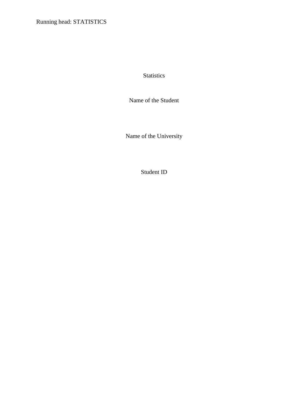
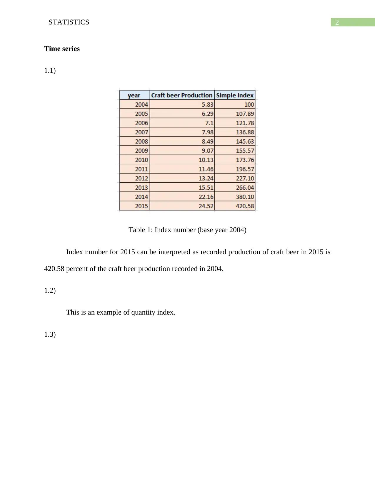
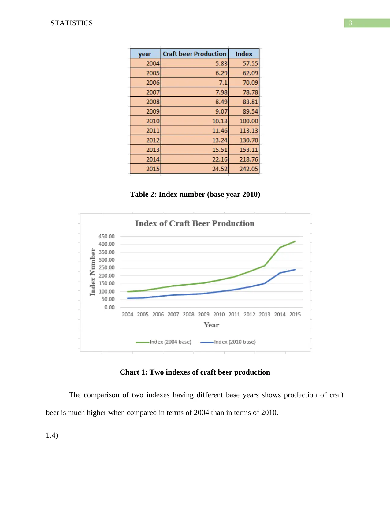
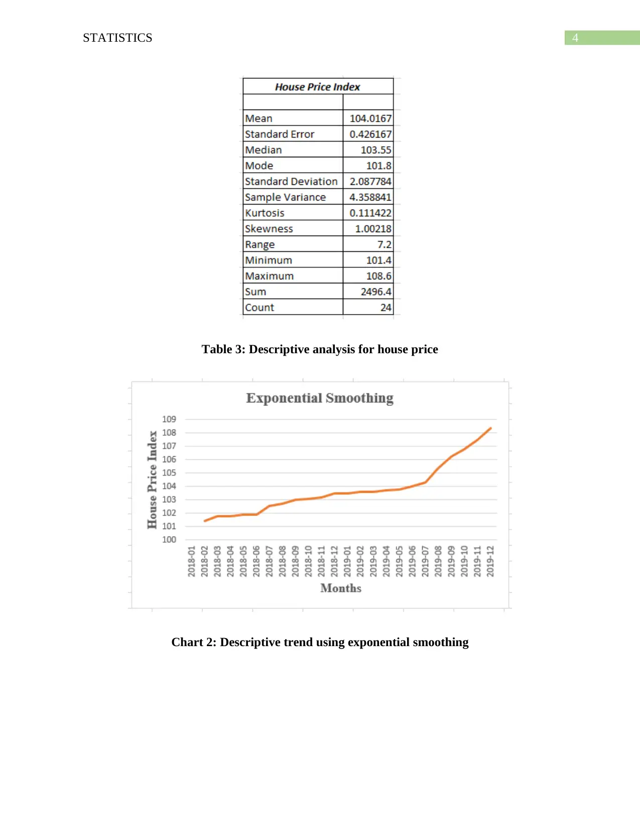
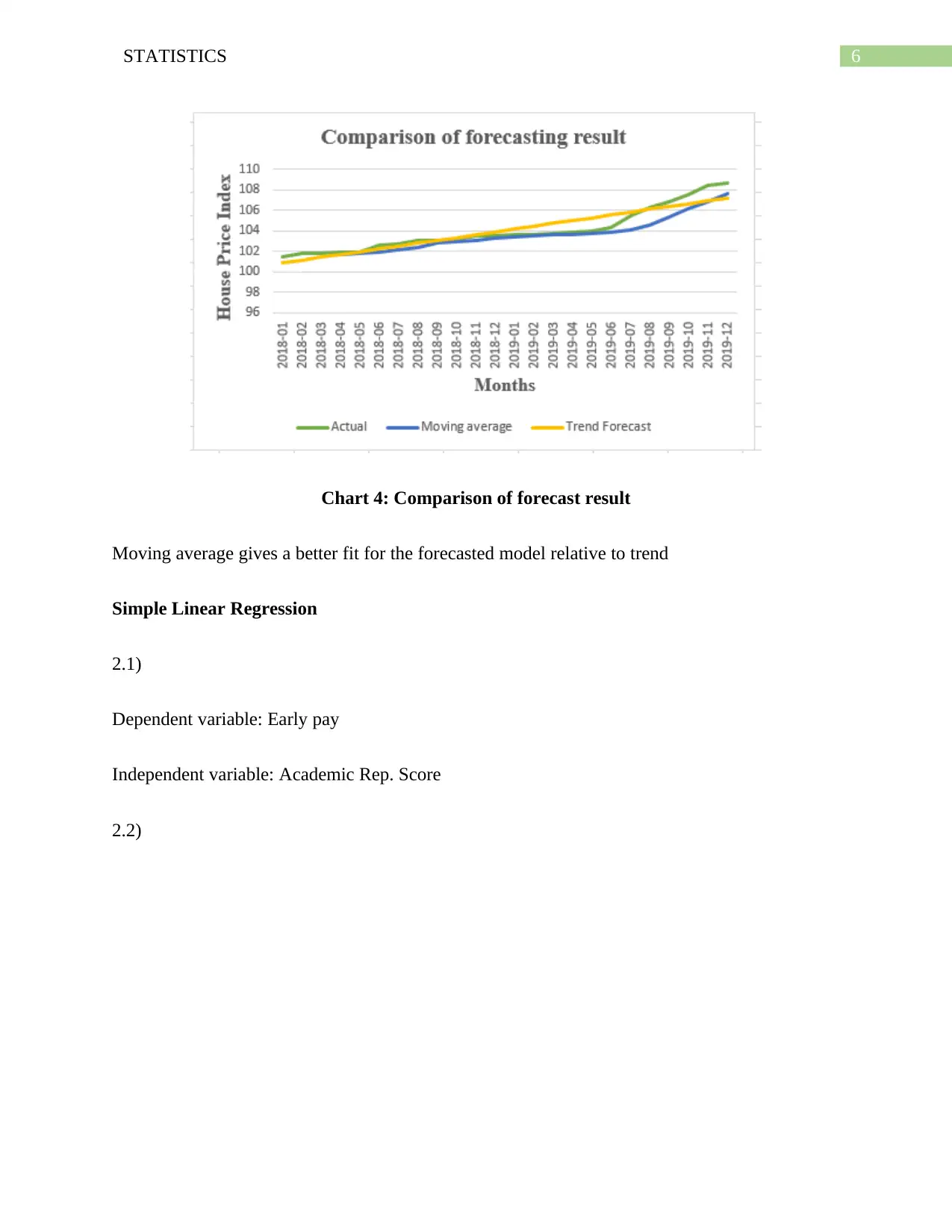
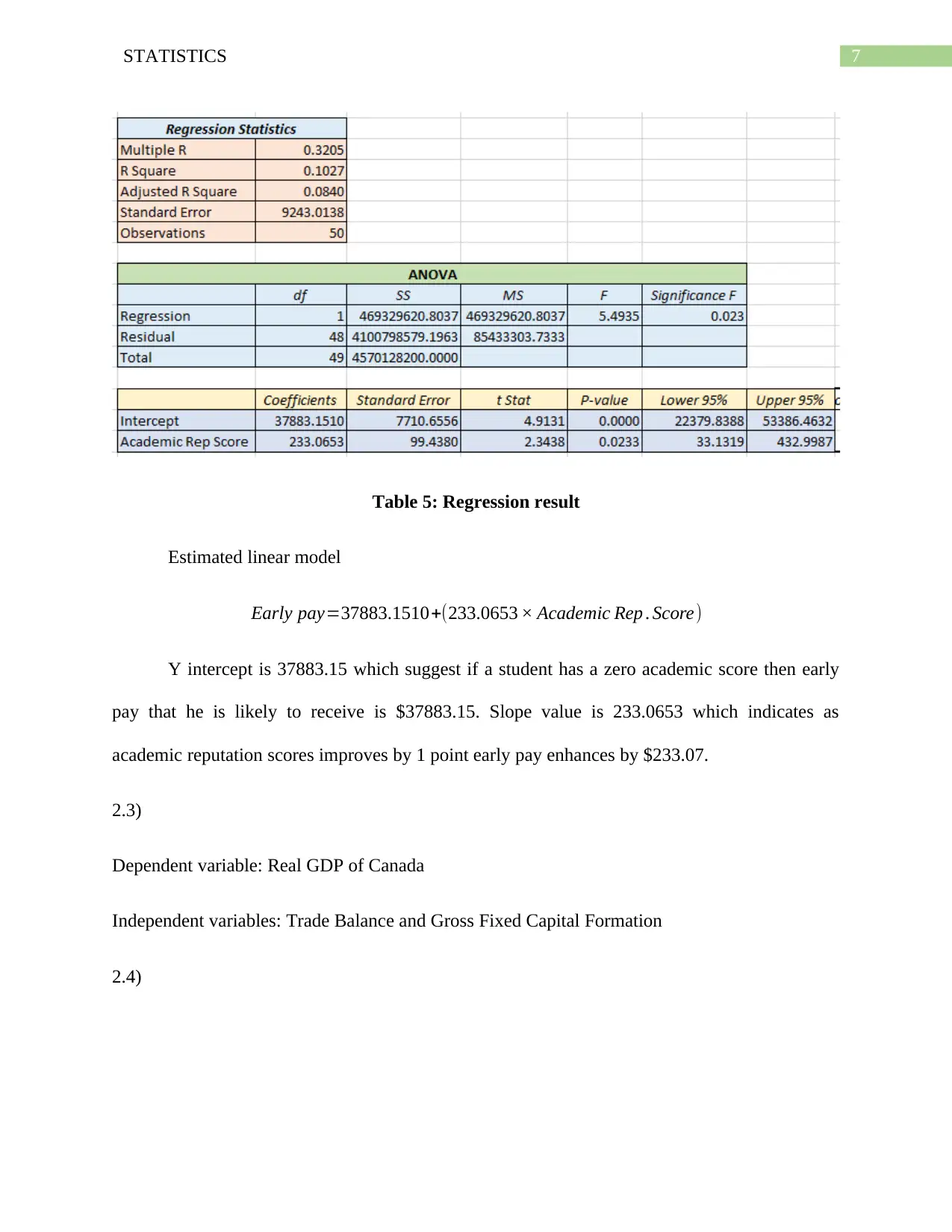
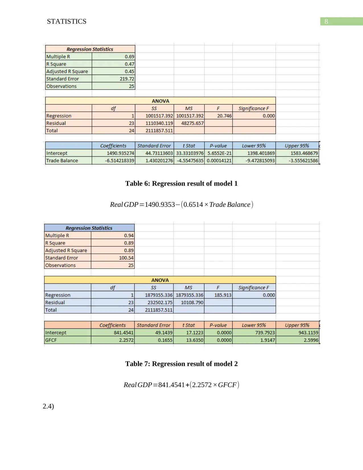
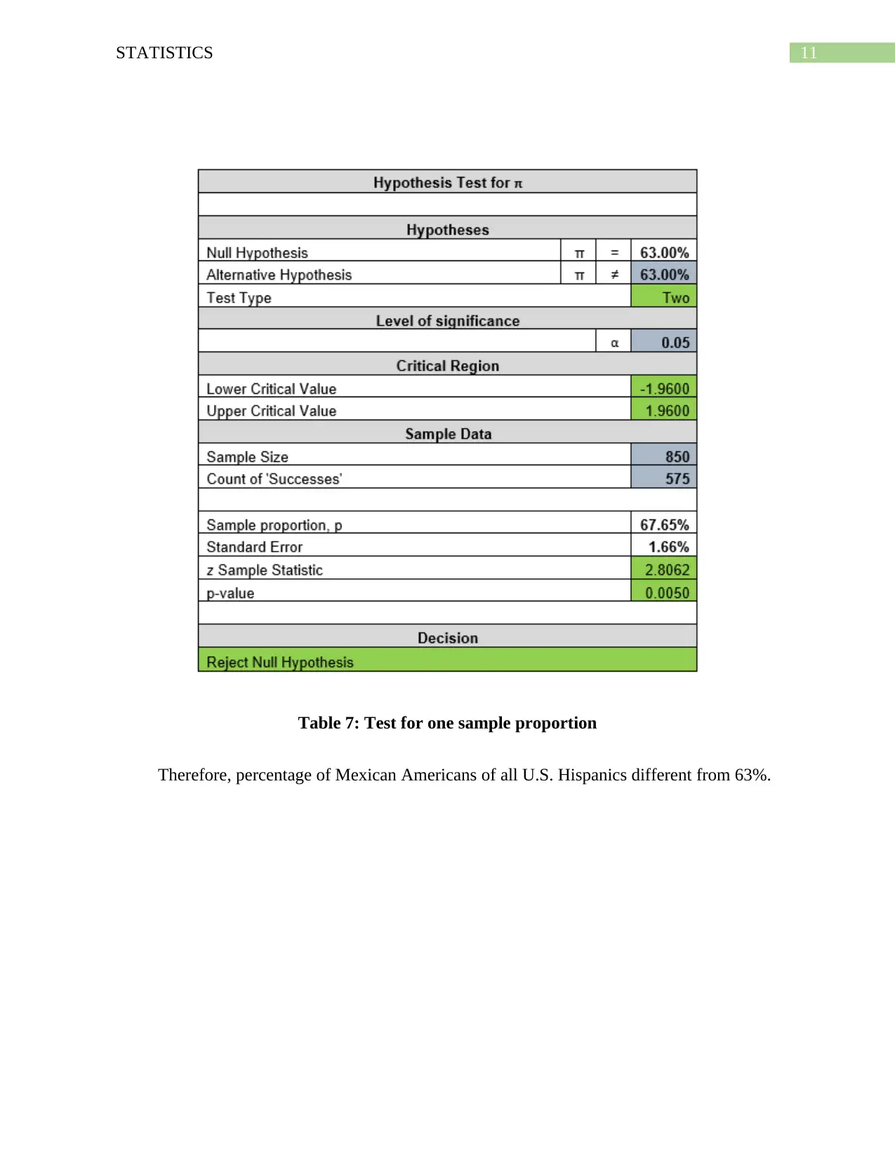
This statistics assignment analyzes time series data, performs regression analysis, and conducts hypothesis tests. The assignment begins with an analysis of U.S. craft beer production from 2004 to 2015, calculating index numbers and interpreting the results. It then moves on to a student-provided time series dataset, focusing on descriptive analysis and trend identification using exponential smoothing and index numbers. The assignment also covers simple linear regression, examining the relationship between variables like academic reputation and early pay, and between real GDP and trade balance/gross fixed capital formation. Finally, it includes hypothesis testing, performing one-sample proportion and mean tests to draw conclusions about various datasets and scenarios. The student provides tables, charts, and interpretations to support the statistical analyses.

Running head: STATISTICS
Statistics
Name of the Student
Name of the University
Student ID

1STATISTICS
Table of Contents
Time series.......................................................................................................................................2
Simple Linear Regression................................................................................................................6
Hypothesis and Test.......................................................................................................................10

2STATISTICS
Time series
1.1)
Table 1: Index number (base year 2004)
Index number for 2015 can be interpreted as recorded production of craft beer in 2015 is
420.58 percent of the craft beer production recorded in 2004.
1.2)
This is an example of quantity index.
1.3)

3STATISTICS
Table 2: Index number (base year 2010)
Chart 1: Two indexes of craft beer production
The comparison of two indexes having different base years shows production of craft
beer is much higher when compared in terms of 2004 than in terms of 2010.
1.4)

4STATISTICS
Table 3: Descriptive analysis for house price
Chart 2: Descriptive trend using exponential smoothing

5STATISTICS
Chart 3: Descriptive trend using index number
Both exponential and index number shows an upward rising trend for house price
1.5)
Table 4: Forecasted house price index for next year

6STATISTICS
Chart 4: Comparison of forecast result
Moving average gives a better fit for the forecasted model relative to trend
Simple Linear Regression
2.1)
Dependent variable: Early pay
Independent variable: Academic Rep. Score
2.2)

7STATISTICS
Table 5: Regression result
Estimated linear model
Early pay=37883.1510+(233.0653 × Academic Rep . Score)
Y intercept is 37883.15 which suggest if a student has a zero academic score then early
pay that he is likely to receive is $37883.15. Slope value is 233.0653 which indicates as
academic reputation scores improves by 1 point early pay enhances by $233.07.
2.3)
Dependent variable: Real GDP of Canada
Independent variables: Trade Balance and Gross Fixed Capital Formation
2.4)

8STATISTICS
Table 6: Regression result of model 1
Real GDP=1490.9353−(0.6514 ×Trade Balance )
Table 7: Regression result of model 2
Real GDP=841.4541+(2.2572 ×GFCF)
2.4)

9STATISTICS
Sign of estimated slope coefficient is negative for model 1 suggesting an inverse relation
between GDP and trade balance. For model 2, estimated slope is positive meaning a positive
relation between real GDP and gross fixed capital formation.
P value for both the slope coefficient is 0.0000 (less than significance at 5% level)
indicating both the coefficients are statistically significant.
Assumptions
Linearity of parameters
Random sampling technique
Homoscadasticity
Absence of multicollinearity and serial autocorrelation
Normality of error terms.
2.5)
Respective R square values for model 1 and model 2 are 0.47 and 0.89. Gross Fixed
Capital Formation predicts real GDP better than Trade Balance. This variable is necessarily best
in general.

10STATISTICS
Hypothesis and Test
3.1)
a)

11STATISTICS
Table 7: Test for one sample proportion
Therefore, percentage of Mexican Americans of all U.S. Hispanics different from 63%.