Probability and Statistics Assignment Solution - University
VerifiedAdded on 2022/09/26
|16
|367
|21
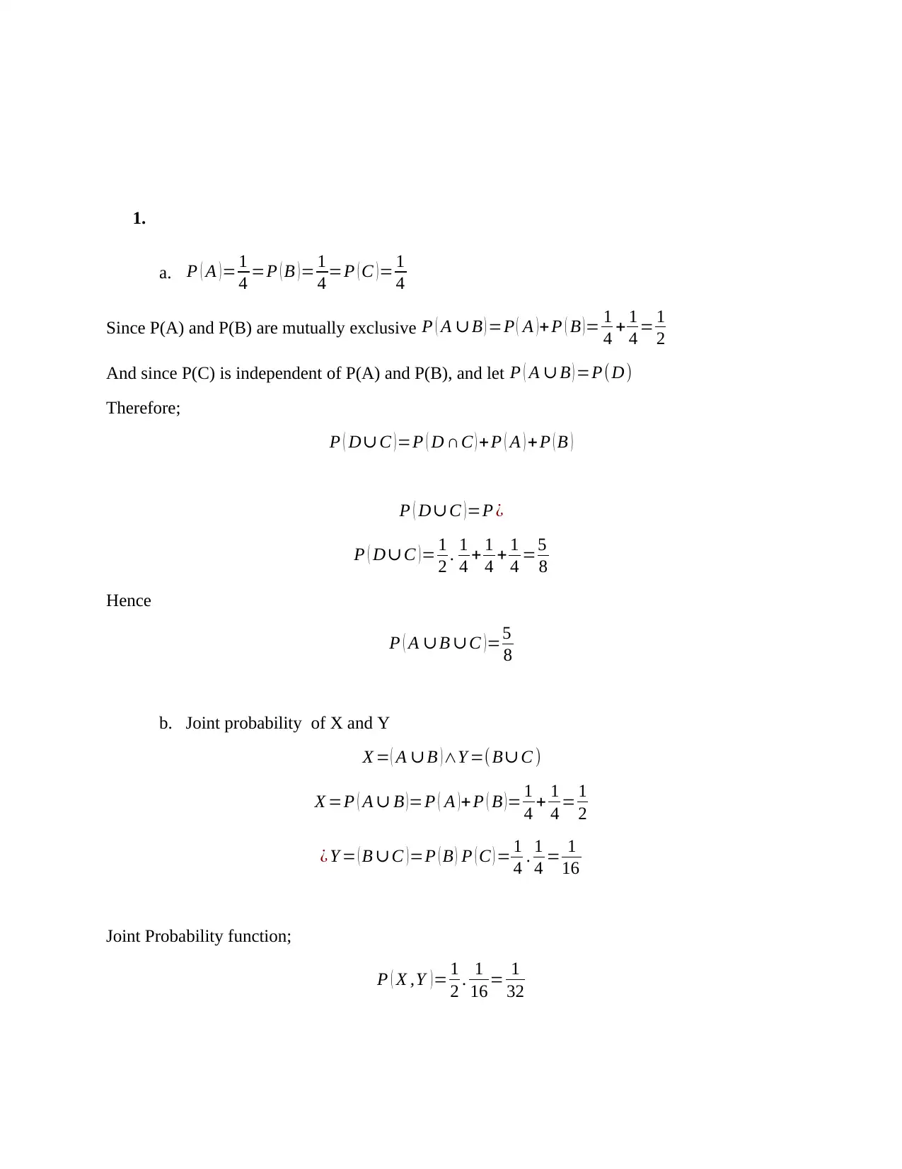
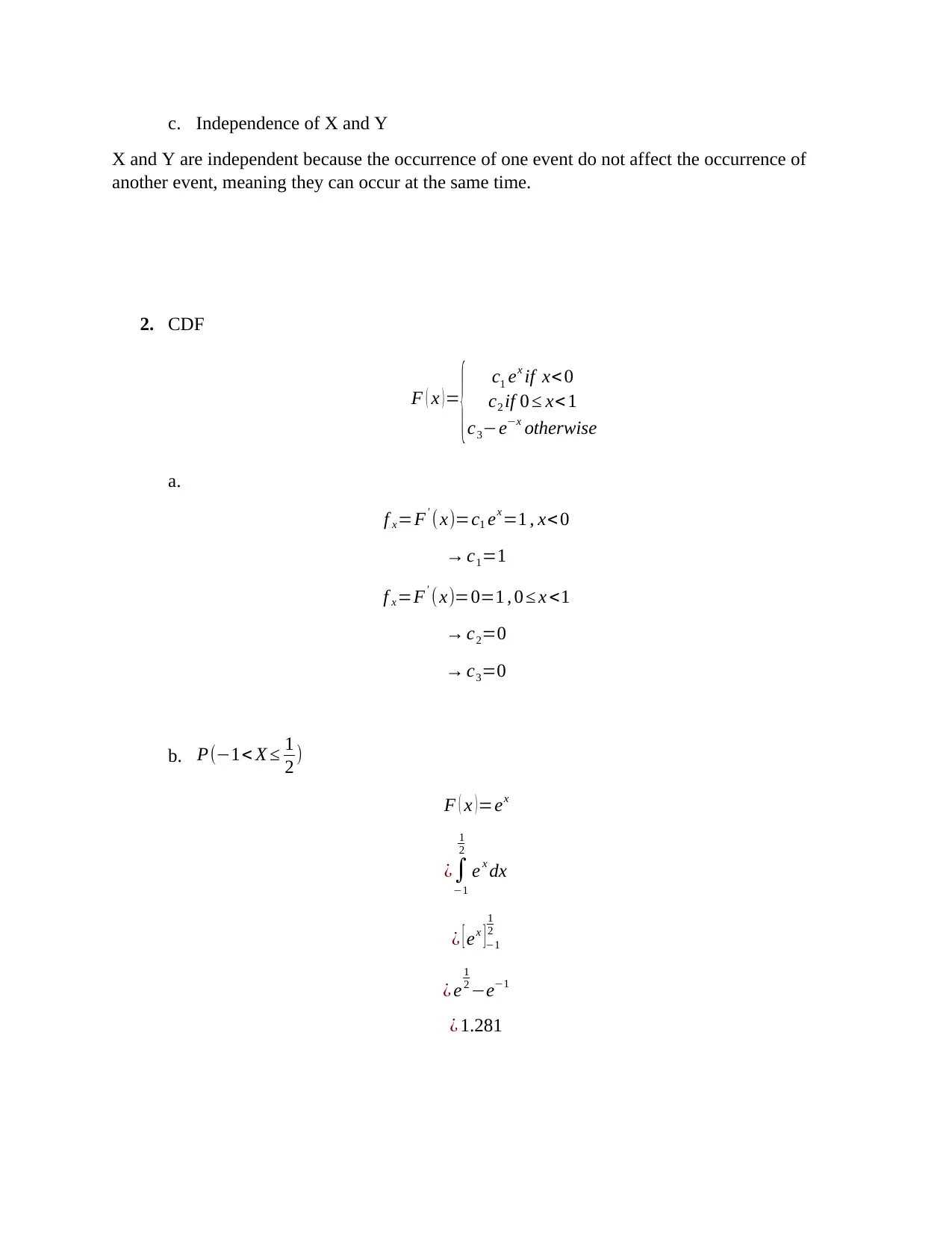
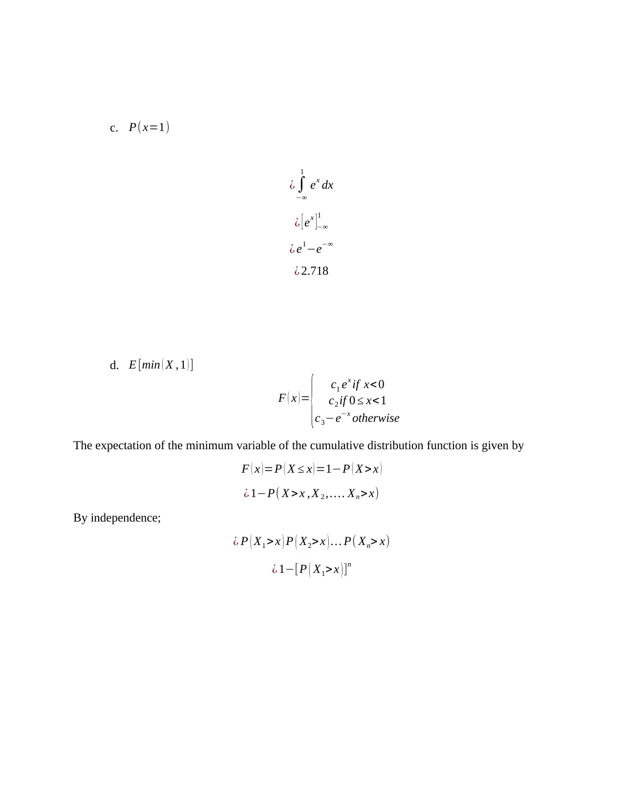
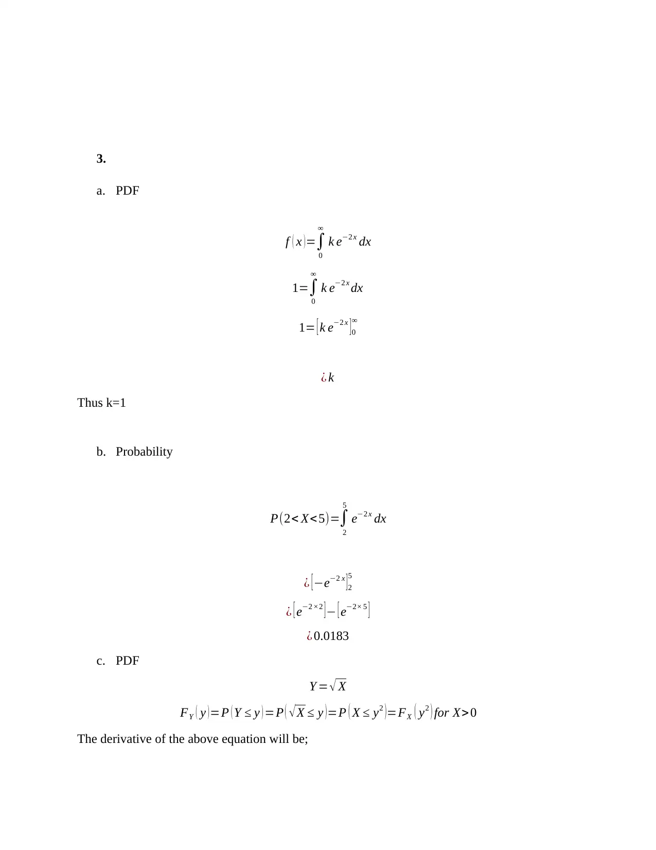
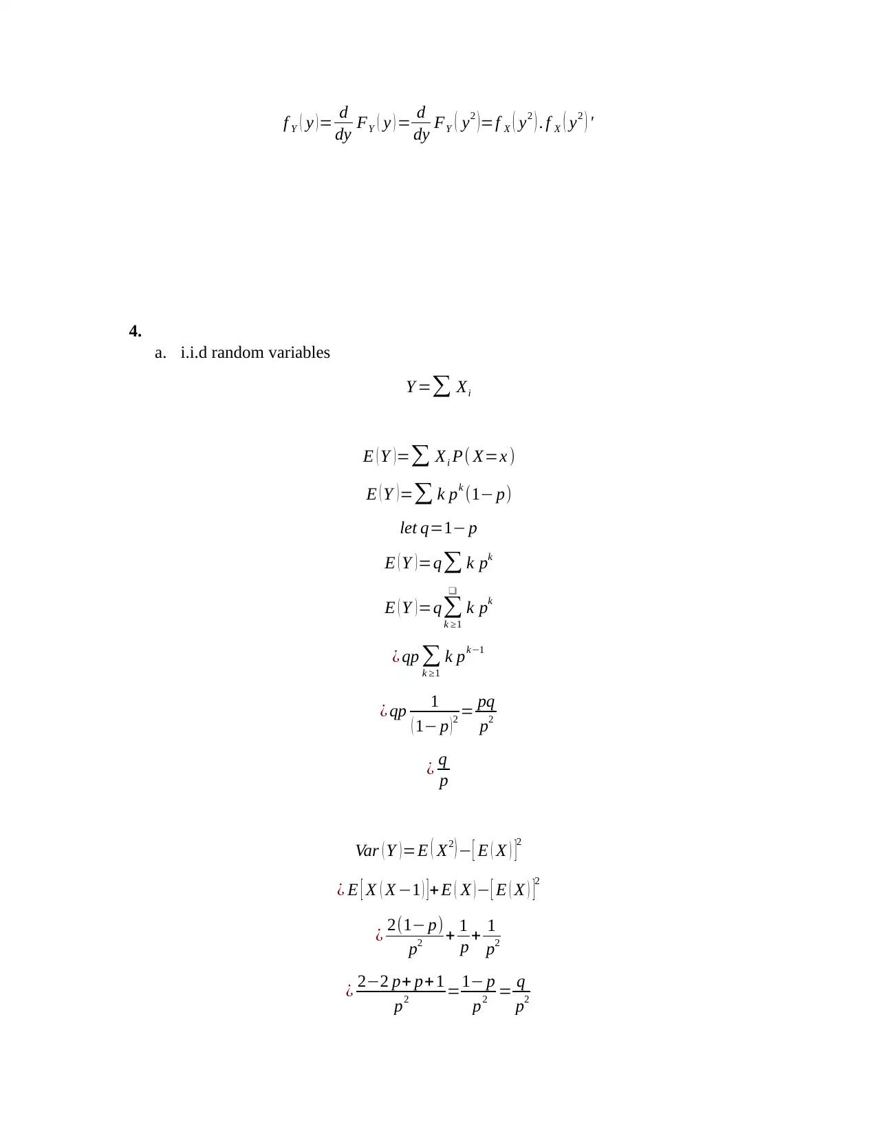
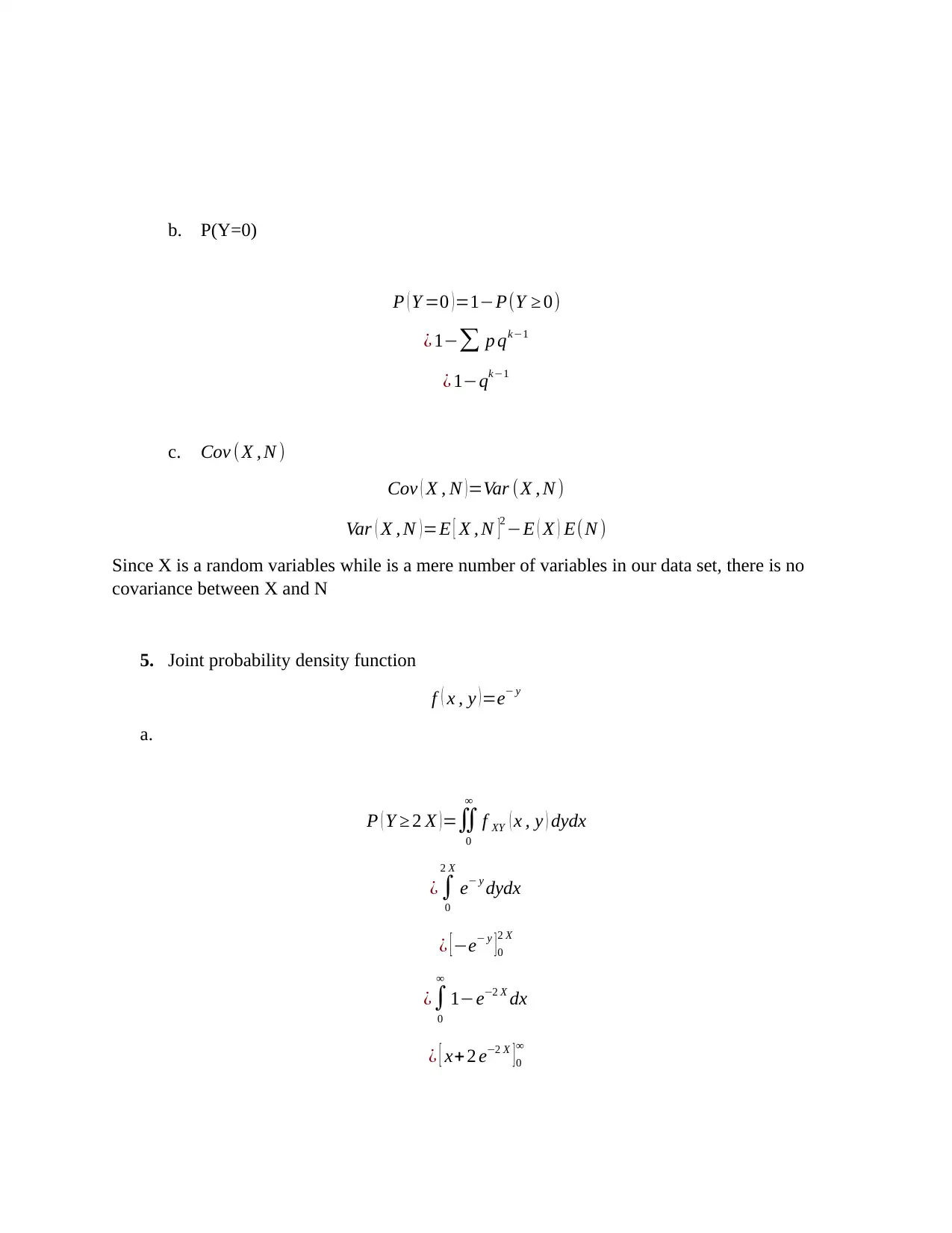
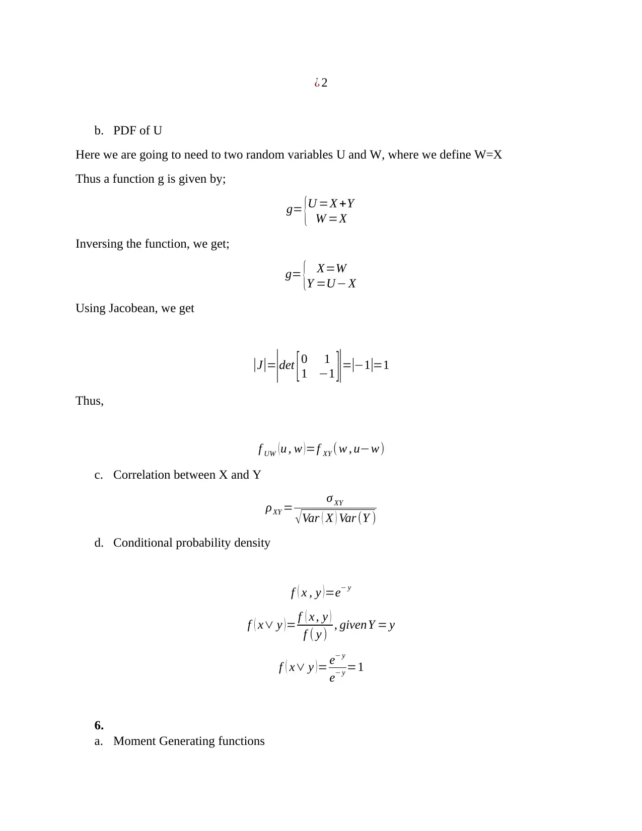
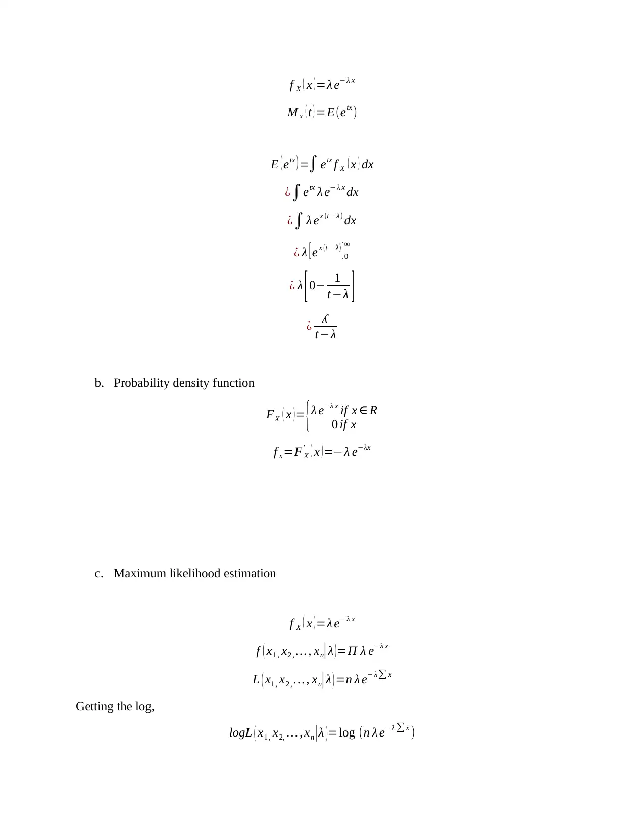
Homework Assignment
AI Summary
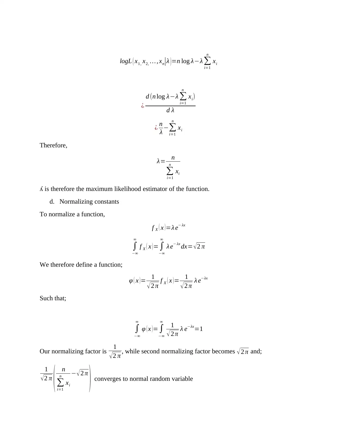
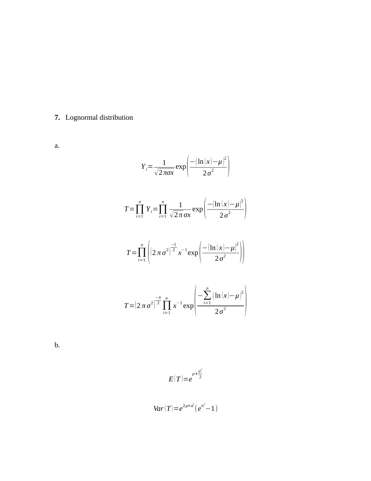
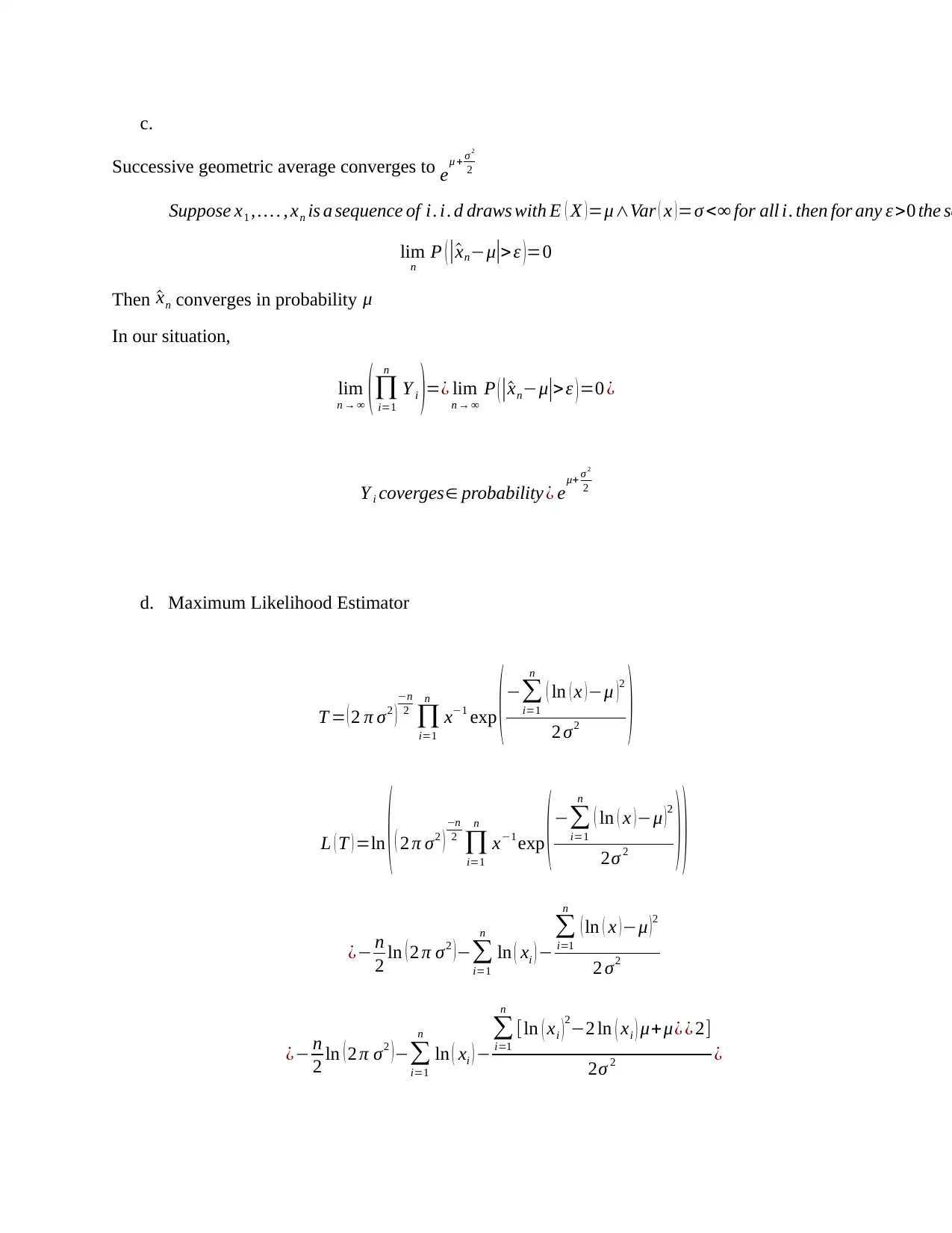
This document presents a comprehensive solution to a probability and statistics homework assignment. The solution covers a wide range of topics, including mutually exclusive events, indicator random variables, cumulative distribution functions, probability density functions, geometric and Poisson distributions, and maximum likelihood estimation. The assignment addresses concepts such as independence, joint probability, conditional probability, moment-generating functions, lognormal distributions, and method of moments estimation. The solutions involve detailed calculations and derivations, providing a thorough understanding of the statistical concepts presented in the assignment. The student has provided all the necessary steps to solve the problems. The document is intended to help students understand and solve similar problems.

1 out of 16
Related Documents


Your All-in-One AI-Powered Toolkit for Academic Success.
+13062052269
info@desklib.com
Available 24*7 on WhatsApp / Email
![[object Object]](/_next/static/media/star-bottom.7253800d.svg)
Copyright © 2020–2026 A2Z Services. All Rights Reserved. Developed and managed by ZUCOL.