Statistics and Probability Homework Assignment Solution

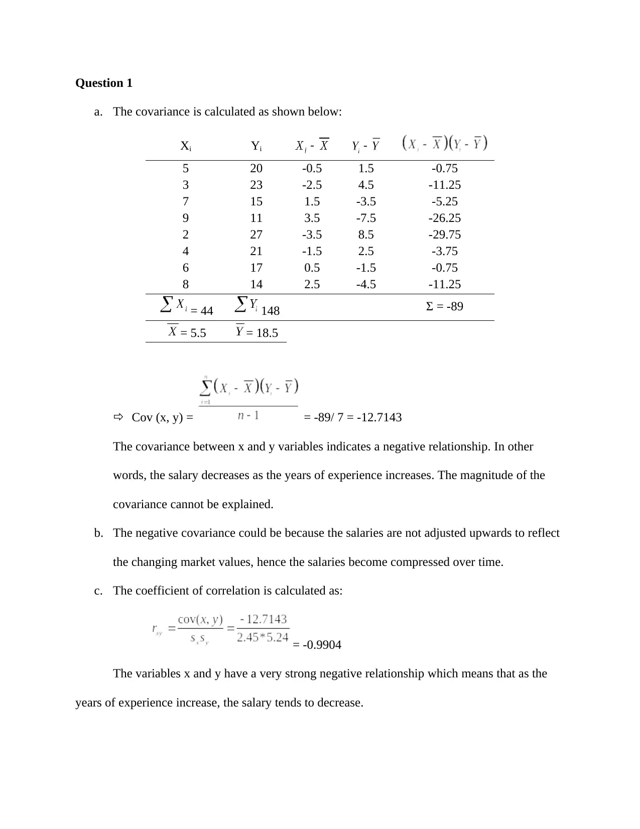
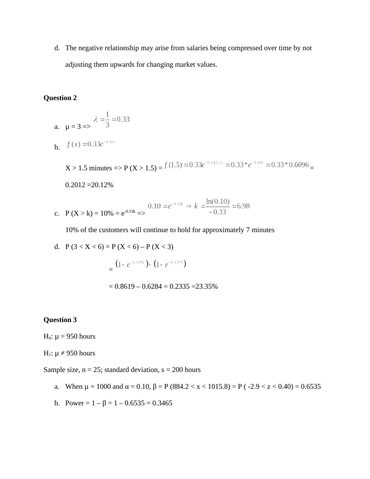
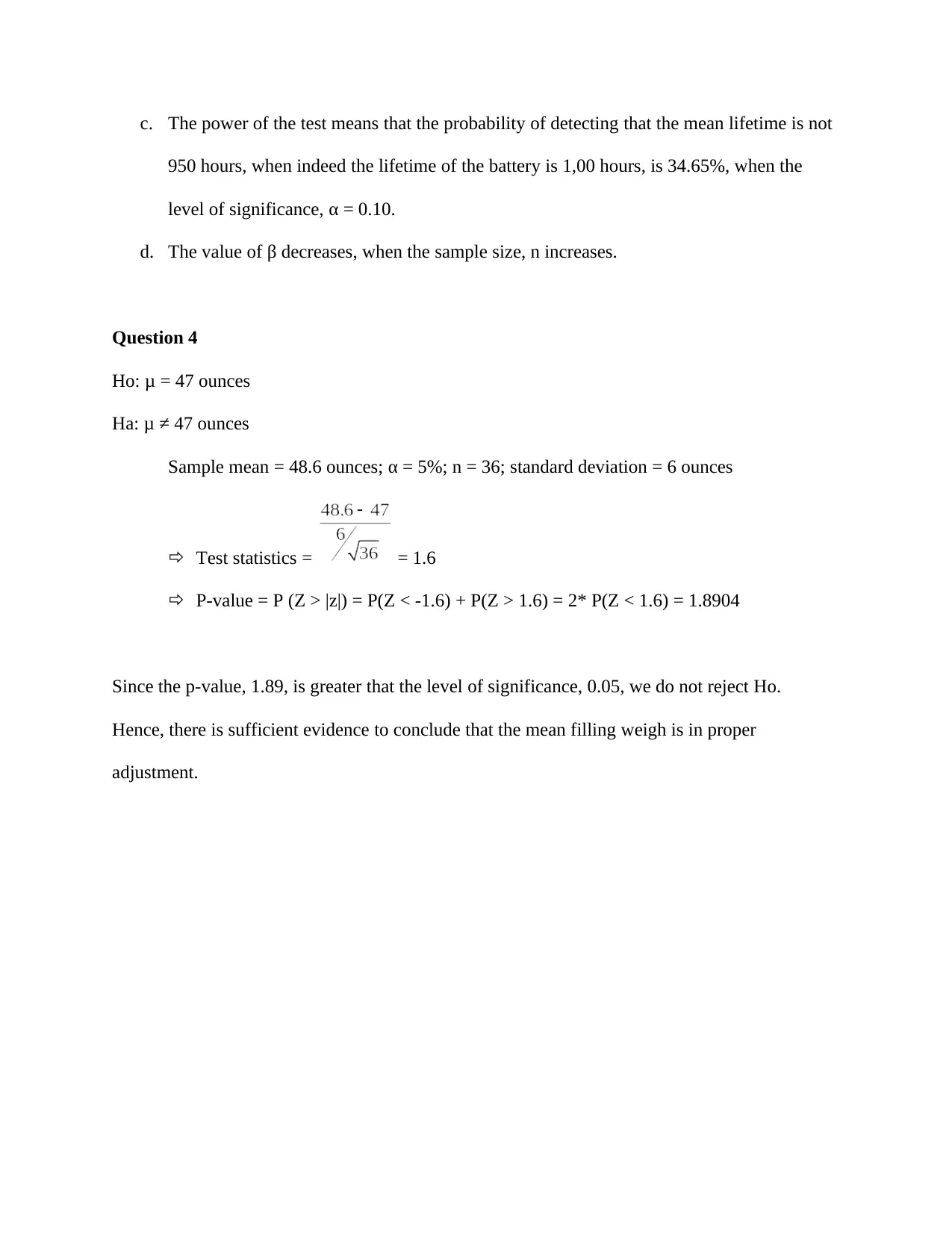
This document presents a detailed solution to a statistics homework assignment, addressing questions related to covariance, correlation, probability distributions, and hypothesis testing. The solution begins with the calculation of covariance and correlation, interpreting the relationship between variables and discussing potential reasons for negative correlation. It then delves into probability calculations using exponential distributions, determining probabilities for customer waiting times. Finally, the assignment explores hypothesis testing, evaluating the power of a test and conducting a hypothesis test to determine if a mean filling weight is in proper adjustment. The solution provides step-by-step calculations and interpretations, offering a comprehensive understanding of the statistical concepts involved.

Question 1
a. The covariance is calculated as shown below:
Xi Yi
5 20 -0.5 1.5 -0.75
3 23 -2.5 4.5 -11.25
7 15 1.5 -3.5 -5.25
9 11 3.5 -7.5 -26.25
2 27 -3.5 8.5 -29.75
4 21 -1.5 2.5 -3.75
6 17 0.5 -1.5 -0.75
8 14 2.5 -4.5 -11.25
= 44 148 Σ = -89
= 5.5 = 18.5
 Cov (x, y) = = -89/ 7 = -12.7143
The covariance between x and y variables indicates a negative relationship. In other
words, the salary decreases as the years of experience increases. The magnitude of the
covariance cannot be explained.
b. The negative covariance could be because the salaries are not adjusted upwards to reflect
the changing market values, hence the salaries become compressed over time.
c. The coefficient of correlation is calculated as:
= -0.9904
The variables x and y have a very strong negative relationship which means that as the
years of experience increase, the salary tends to decrease.

d. The negative relationship may arise from salaries being compressed over time by not
adjusting them upwards for changing market values.
Question 2
a. μ = 3 =>
b.
X > 1.5 minutes => P (X > 1.5) = =
0.2012 =20.12%
c. P (X > k) = 10% = e-0.33k =>
10% of the customers will continue to hold for approximately 7 minutes
d. P (3 < X < 6) = P (X < 6) – P (X < 3)
=
= 0.8619 – 0.6284 = 0.2335 =23.35%
Question 3
H0: μ = 950 hours
H1: μ ≠ 950 hours
Sample size, n = 25; standard deviation, s = 200 hours
a. When μ = 1000 and α = 0.10, β = P (884.2 < x < 1015.8) = P ( -2.9 < z < 0.40) = 0.6535
b. Power = 1 – β = 1 – 0.6535 = 0.3465

c. The power of the test means that the probability of detecting that the mean lifetime is not
950 hours, when indeed the lifetime of the battery is 1,00 hours, is 34.65%, when the
level of significance, α = 0.10.
d. The value of β decreases, when the sample size, n increases.
Question 4
Ho: μ = 47 ounces
Ha: μ ≠ 47 ounces
Sample mean = 48.6 ounces; α = 5%; n = 36; standard deviation = 6 ounces
 Test statistics = = 1.6
 P-value = P (Z > |z|) = P(Z < -1.6) + P(Z > 1.6) = 2* P(Z < 1.6) = 1.8904
Since the p-value, 1.89, is greater that the level of significance, 0.05, we do not reject Ho.
Hence, there is sufficient evidence to conclude that the mean filling weigh is in proper
adjustment.