Statistical Analysis Homework: Probability, Distributions, and Tests

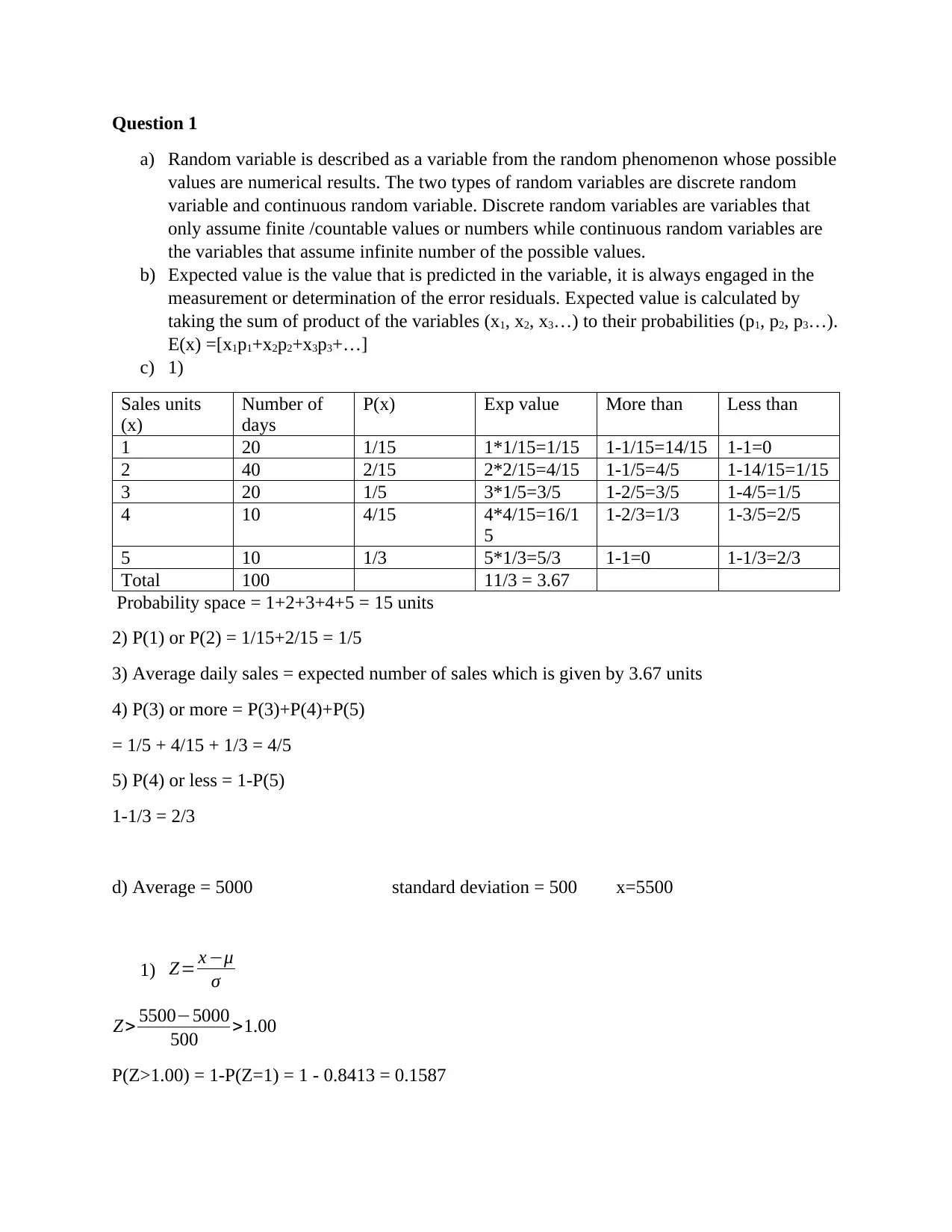
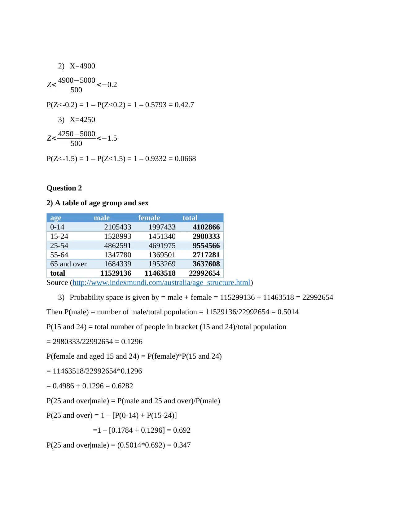
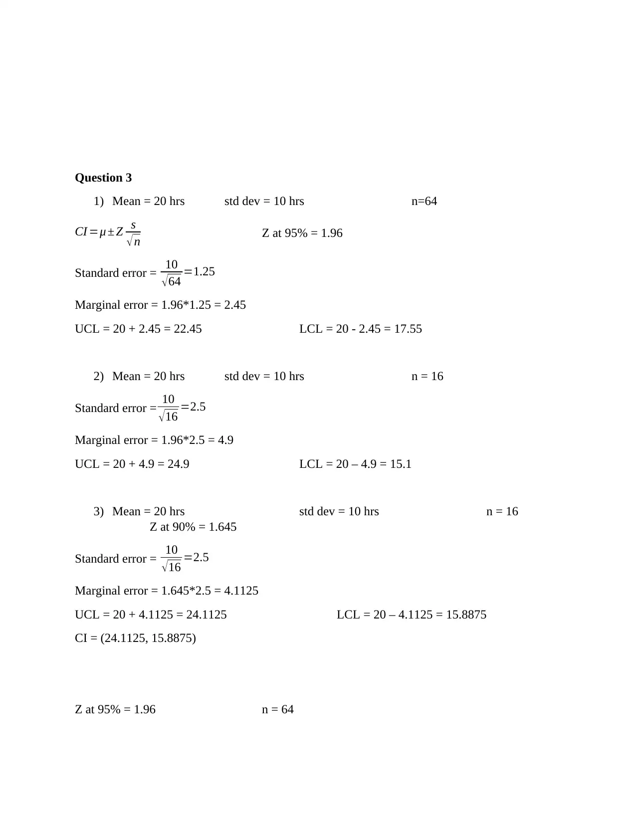
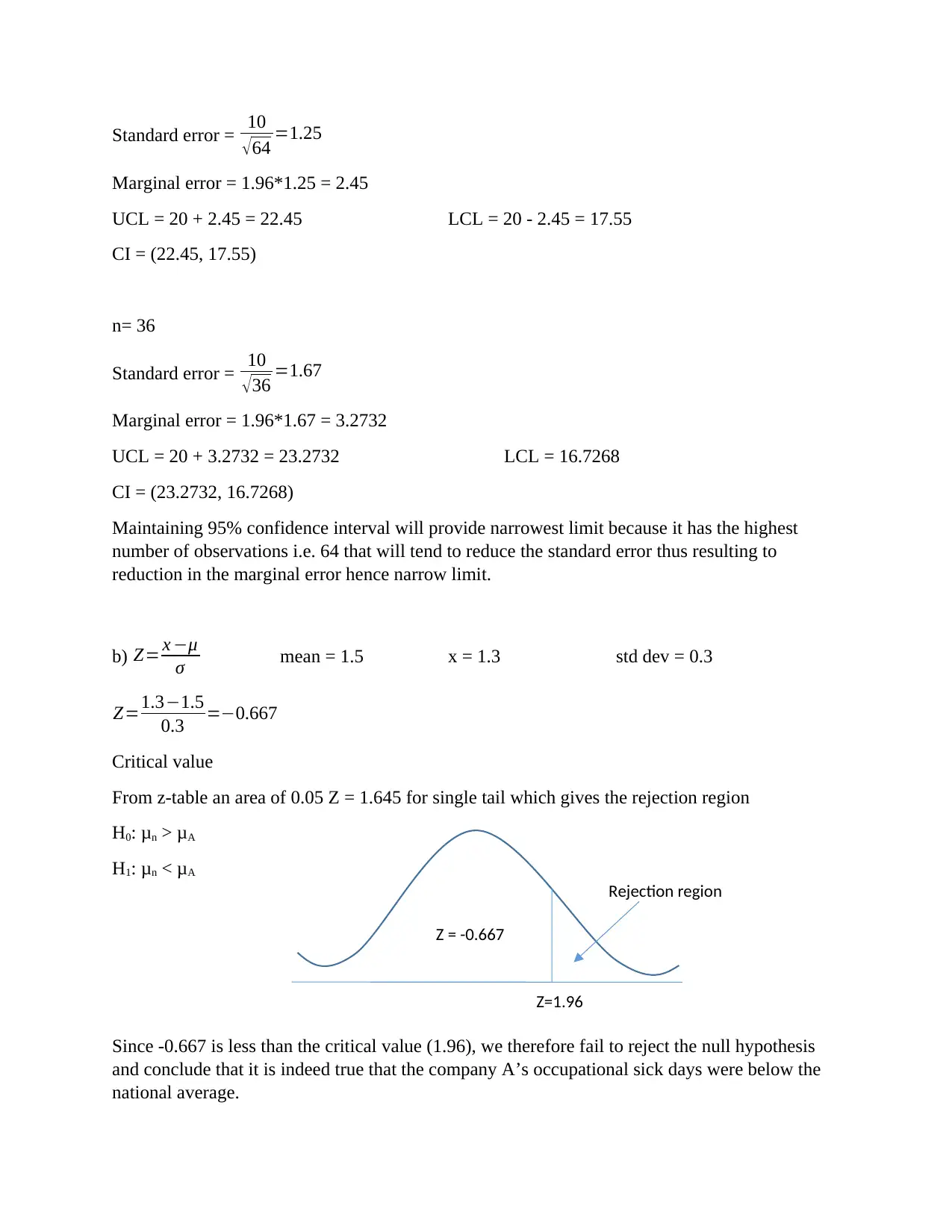
This homework assignment provides solutions to three statistical problems. The first problem explores random variables, including discrete and continuous types, and calculates expected values, probabilities, and average daily sales based on a given sales distribution. The second problem delves into probability calculations using demographic data, determining probabilities for various age and gender groups. The third problem focuses on confidence intervals and hypothesis testing, calculating confidence intervals for different sample sizes and confidence levels and performing a one-tailed hypothesis test to compare a company's occupational sick days to the national average. The solutions demonstrate the application of key statistical concepts and formulas.

Question 1
a) Random variable is described as a variable from the random phenomenon whose possible
values are numerical results. The two types of random variables are discrete random
variable and continuous random variable. Discrete random variables are variables that
only assume finite /countable values or numbers while continuous random variables are
the variables that assume infinite number of the possible values.
b) Expected value is the value that is predicted in the variable, it is always engaged in the
measurement or determination of the error residuals. Expected value is calculated by
taking the sum of product of the variables (x1, x2, x3…) to their probabilities (p1, p2, p3…).
E(x) =[x1p1+x2p2+x3p3+…]
c) 1)
Sales units
(x)
Number of
days
P(x) Exp value More than Less than
1 20 1/15 1*1/15=1/15 1-1/15=14/15 1-1=0
2 40 2/15 2*2/15=4/15 1-1/5=4/5 1-14/15=1/15
3 20 1/5 3*1/5=3/5 1-2/5=3/5 1-4/5=1/5
4 10 4/15 4*4/15=16/1
5
1-2/3=1/3 1-3/5=2/5
5 10 1/3 5*1/3=5/3 1-1=0 1-1/3=2/3
Total 100 11/3 = 3.67
Probability space = 1+2+3+4+5 = 15 units
2) P(1) or P(2) = 1/15+2/15 = 1/5
3) Average daily sales = expected number of sales which is given by 3.67 units
4) P(3) or more = P(3)+P(4)+P(5)
= 1/5 + 4/15 + 1/3 = 4/5
5) P(4) or less = 1-P(5)
1-1/3 = 2/3
d) Average = 5000 standard deviation = 500 x=5500
1) Z= x −μ
σ
Z> 5500−5000
500 >1.00
P(Z>1.00) = 1-P(Z=1) = 1 - 0.8413 = 0.1587

2) X=4900
Z< 4900−5000
500 <−0.2
P(Z<-0.2) = 1 – P(Z<0.2) = 1 – 0.5793 = 0.42.7
3) X=4250
Z< 4250−5000
500 <−1.5
P(Z<-1.5) = 1 – P(Z<1.5) = 1 – 0.9332 = 0.0668
Question 2
2) A table of age group and sex
age male female total
0-14 2105433 1997433 4102866
15-24 1528993 1451340 2980333
25-54 4862591 4691975 9554566
55-64 1347780 1369501 2717281
65 and over 1684339 1953269 3637608
total 11529136 11463518 22992654
Source (http://www.indexmundi.com/australia/age_structure.html)
3) Probability space is given by = male + female = 115299136 + 11463518 = 22992654
Then P(male) = number of male/total population = 11529136/22992654 = 0.5014
P(15 and 24) = total number of people in bracket (15 and 24)/total population
= 2980333/22992654 = 0.1296
P(female and aged 15 and 24) = P(female)*P(15 and 24)
= 11463518/22992654*0.1296
= 0.4986 + 0.1296 = 0.6282
P(25 and over|male) = P(male and 25 and over)/P(male)
P(25 and over) = 1 – [P(0-14) + P(15-24)]
=1 – [0.1784 + 0.1296] = 0.692
P(25 and over|male) = (0.5014*0.692) = 0.347

Question 3
1) Mean = 20 hrs std dev = 10 hrs n=64
CI =μ ± Z s
√n Z at 95% = 1.96
Standard error = 10
√64 =1.25
Marginal error = 1.96*1.25 = 2.45
UCL = 20 + 2.45 = 22.45 LCL = 20 - 2.45 = 17.55
2) Mean = 20 hrs std dev = 10 hrs n = 16
Standard error = 10
√16 =2.5
Marginal error = 1.96*2.5 = 4.9
UCL = 20 + 4.9 = 24.9 LCL = 20 – 4.9 = 15.1
3) Mean = 20 hrs std dev = 10 hrs n = 16
Z at 90% = 1.645
Standard error = 10
√16 =2.5
Marginal error = 1.645*2.5 = 4.1125
UCL = 20 + 4.1125 = 24.1125 LCL = 20 – 4.1125 = 15.8875
CI = (24.1125, 15.8875)
Z at 95% = 1.96 n = 64

Standard error = 10
√64 =1.25
Marginal error = 1.96*1.25 = 2.45
UCL = 20 + 2.45 = 22.45 LCL = 20 - 2.45 = 17.55
CI = (22.45, 17.55)
n= 36
Standard error = 10
√36 =1.67
Marginal error = 1.96*1.67 = 3.2732
UCL = 20 + 3.2732 = 23.2732 LCL = 16.7268
CI = (23.2732, 16.7268)
Maintaining 95% confidence interval will provide narrowest limit because it has the highest
number of observations i.e. 64 that will tend to reduce the standard error thus resulting to
reduction in the marginal error hence narrow limit.
b) Z= x −μ
σ mean = 1.5 x = 1.3 std dev = 0.3
Z=1.3−1.5
0.3 =−0.667
Critical value
From z-table an area of 0.05 Z = 1.645 for single tail which gives the rejection region
H0: μn > μA
H1: μn < μA
Since -0.667 is less than the critical value (1.96), we therefore fail to reject the null hypothesis
and conclude that it is indeed true that the company A’s occupational sick days were below the
national average.
Z = -0.667
Rejection region
Z=1.96