Statistics Homework: Analyzing Household Expenditure Data with Excel

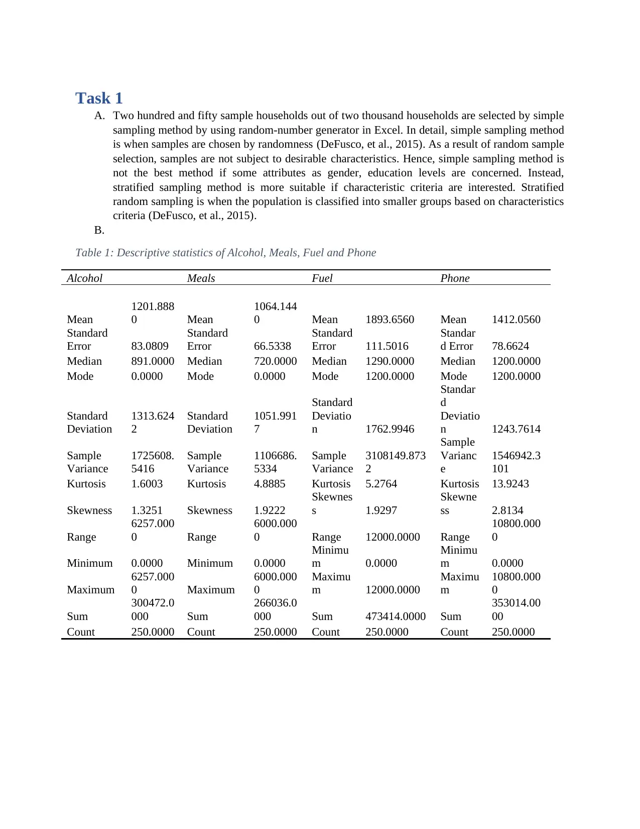
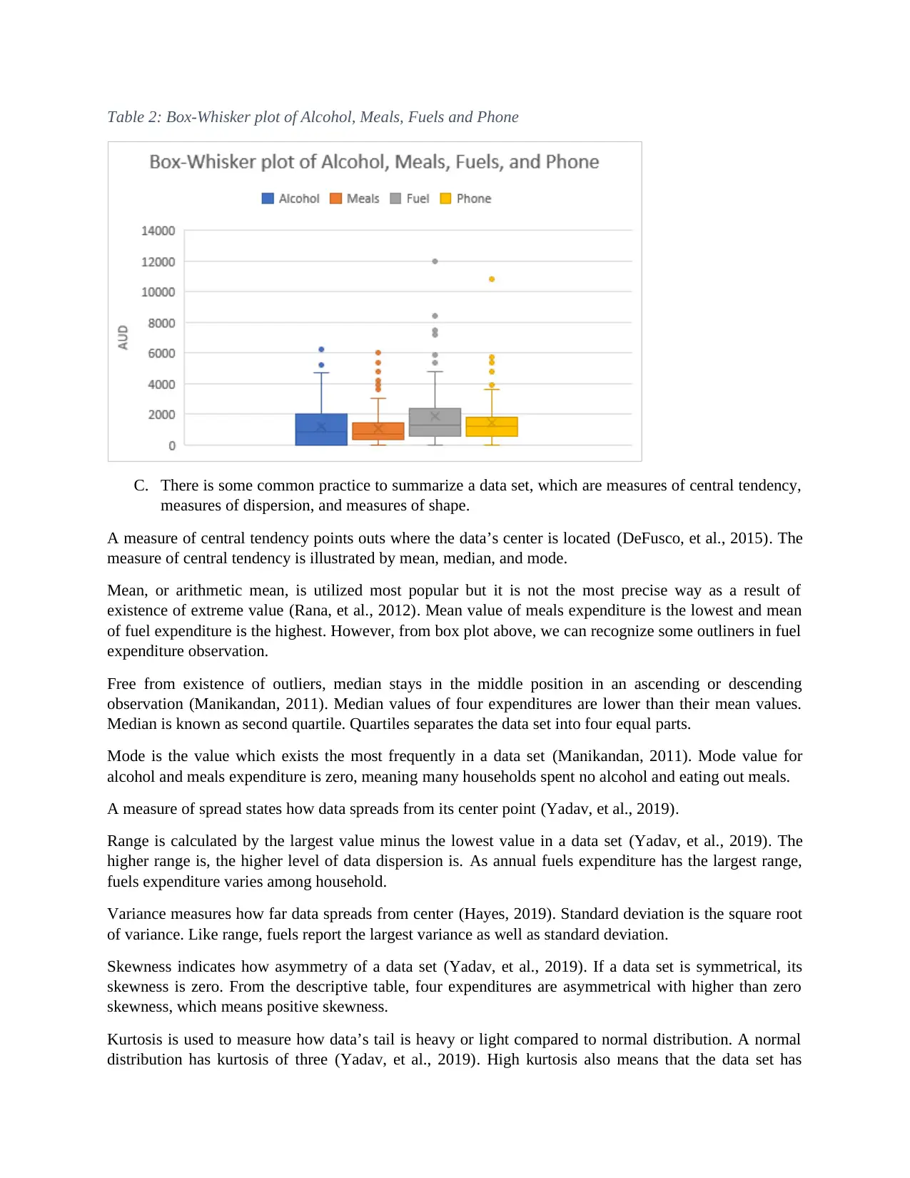
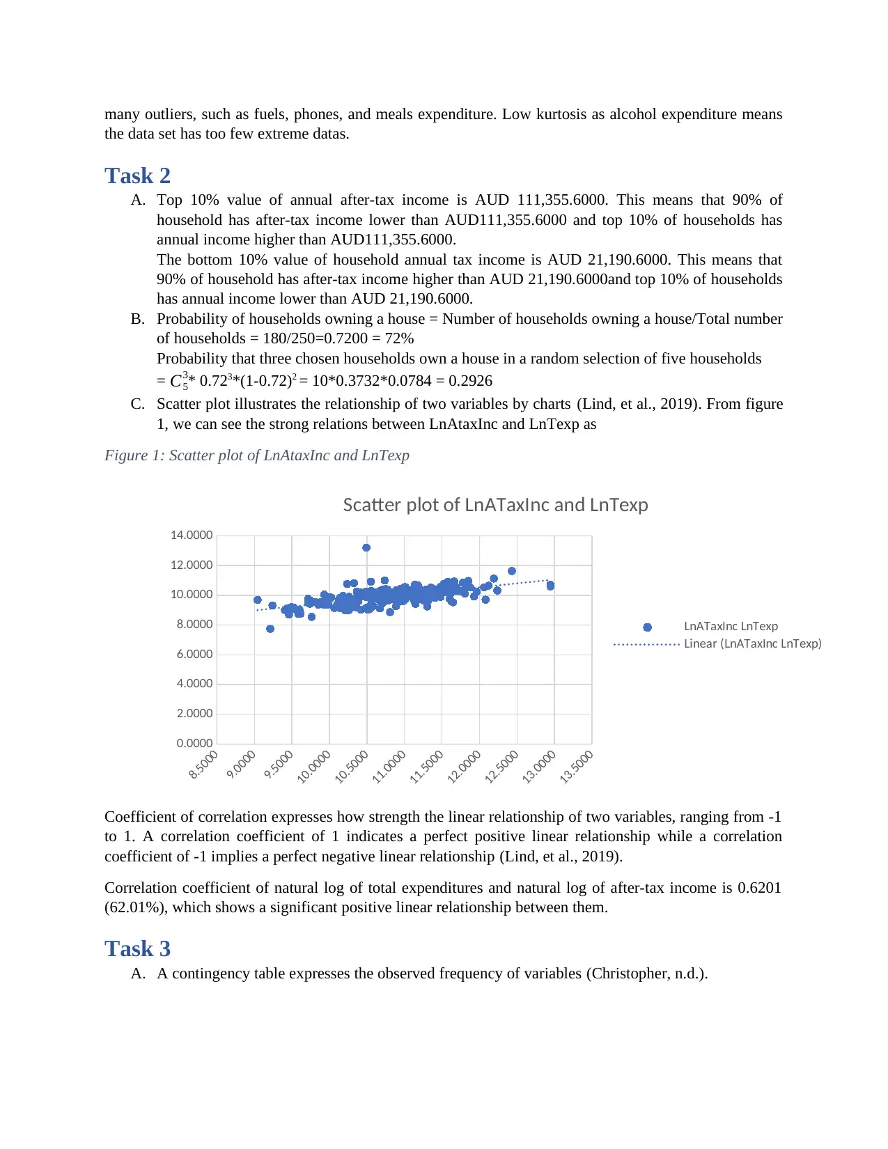
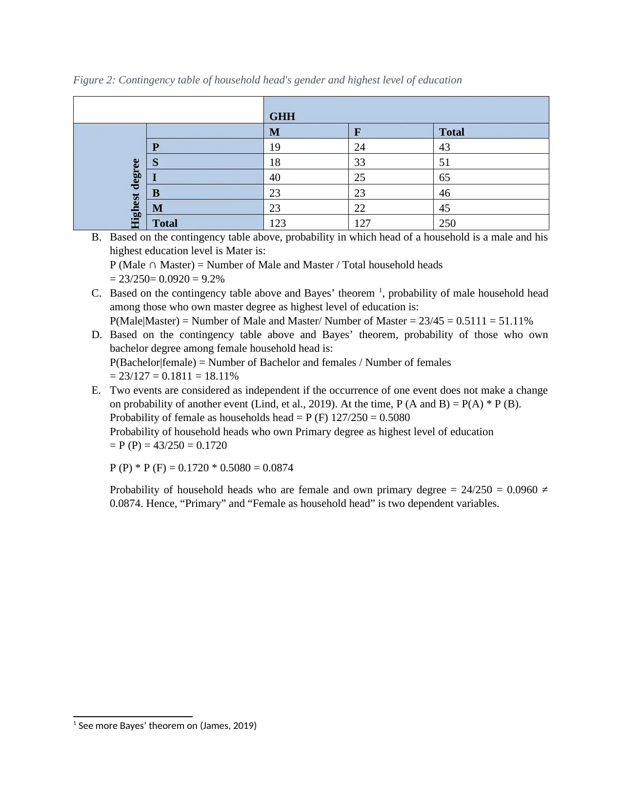
This assignment provides a comprehensive statistical analysis of household expenditure data. It begins with a simple random sampling of 250 households from a larger dataset to analyze expenditures on alcohol, meals, fuel, and phone services. Descriptive statistics, including mean, median, mode, standard deviation, skewness, and kurtosis, are calculated and interpreted to understand the central tendency, dispersion, and shape of the data. The assignment also determines the top and bottom 10% values of after-tax income, calculates the probability of households owning a house, and examines the relationship between after-tax income and total expenditure using scatter plots and correlation coefficients. Finally, it uses a contingency table to analyze the relationship between household head gender and education level, calculating conditional probabilities and determining the independence of variables using Bayes’ theorem. The analysis is supported by tables and figures generated using Excel.

Student’s name: Phuc Thang Nguyen
Student’s ID: 20170603
Word count: 1147 words

Table of Contents
Task 1..........................................................................................................................................................3
Task 2..........................................................................................................................................................5
Task 3..........................................................................................................................................................5
Table of Figures and Tables
Figure 1: Scatter plot of LnAtaxInc and LnTexp.........................................................................................5
Figure 2: Contingency table of household head's gender and highest level of education.............................6
Table 1: Descriptive statistics of Alcohol, Meals, Fuel and Phone..............................................................3
Table 2: Box-Whisker plot of Alcohol, Meals, Fuels and Phone.................................................................4

Task 1
A. Two hundred and fifty sample households out of two thousand households are selected by simple
sampling method by using random-number generator in Excel. In detail, simple sampling method
is when samples are chosen by randomness (DeFusco, et al., 2015). As a result of random sample
selection, samples are not subject to desirable characteristics. Hence, simple sampling method is
not the best method if some attributes as gender, education levels are concerned. Instead,
stratified sampling method is more suitable if characteristic criteria are interested. Stratified
random sampling is when the population is classified into smaller groups based on characteristics
criteria (DeFusco, et al., 2015).
B.
Table 1: Descriptive statistics of Alcohol, Meals, Fuel and Phone
Alcohol Meals Fuel Phone
Mean
1201.888
0 Mean
1064.144
0 Mean 1893.6560 Mean 1412.0560
Standard
Error 83.0809
Standard
Error 66.5338
Standard
Error 111.5016
Standar
d Error 78.6624
Median 891.0000 Median 720.0000 Median 1290.0000 Median 1200.0000
Mode 0.0000 Mode 0.0000 Mode 1200.0000 Mode 1200.0000
Standard
Deviation
1313.624
2
Standard
Deviation
1051.991
7
Standard
Deviatio
n 1762.9946
Standar
d
Deviatio
n 1243.7614
Sample
Variance
1725608.
5416
Sample
Variance
1106686.
5334
Sample
Variance
3108149.873
2
Sample
Varianc
e
1546942.3
101
Kurtosis 1.6003 Kurtosis 4.8885 Kurtosis 5.2764 Kurtosis 13.9243
Skewness 1.3251 Skewness 1.9222
Skewnes
s 1.9297
Skewne
ss 2.8134
Range
6257.000
0 Range
6000.000
0 Range 12000.0000 Range
10800.000
0
Minimum 0.0000 Minimum 0.0000
Minimu
m 0.0000
Minimu
m 0.0000
Maximum
6257.000
0 Maximum
6000.000
0
Maximu
m 12000.0000
Maximu
m
10800.000
0
Sum
300472.0
000 Sum
266036.0
000 Sum 473414.0000 Sum
353014.00
00
Count 250.0000 Count 250.0000 Count 250.0000 Count 250.0000

Table 2: Box-Whisker plot of Alcohol, Meals, Fuels and Phone
C. There is some common practice to summarize a data set, which are measures of central tendency,
measures of dispersion, and measures of shape.
A measure of central tendency points outs where the data’s center is located (DeFusco, et al., 2015). The
measure of central tendency is illustrated by mean, median, and mode.
Mean, or arithmetic mean, is utilized most popular but it is not the most precise way as a result of
existence of extreme value (Rana, et al., 2012). Mean value of meals expenditure is the lowest and mean
of fuel expenditure is the highest. However, from box plot above, we can recognize some outliners in fuel
expenditure observation.
Free from existence of outliers, median stays in the middle position in an ascending or descending
observation (Manikandan, 2011). Median values of four expenditures are lower than their mean values.
Median is known as second quartile. Quartiles separates the data set into four equal parts.
Mode is the value which exists the most frequently in a data set (Manikandan, 2011). Mode value for
alcohol and meals expenditure is zero, meaning many households spent no alcohol and eating out meals.
A measure of spread states how data spreads from its center point (Yadav, et al., 2019).
Range is calculated by the largest value minus the lowest value in a data set (Yadav, et al., 2019). The
higher range is, the higher level of data dispersion is. As annual fuels expenditure has the largest range,
fuels expenditure varies among household.
Variance measures how far data spreads from center (Hayes, 2019). Standard deviation is the square root
of variance. Like range, fuels report the largest variance as well as standard deviation.
Skewness indicates how asymmetry of a data set (Yadav, et al., 2019). If a data set is symmetrical, its
skewness is zero. From the descriptive table, four expenditures are asymmetrical with higher than zero
skewness, which means positive skewness.
Kurtosis is used to measure how data’s tail is heavy or light compared to normal distribution. A normal
distribution has kurtosis of three (Yadav, et al., 2019). High kurtosis also means that the data set has

many outliers, such as fuels, phones, and meals expenditure. Low kurtosis as alcohol expenditure means
the data set has too few extreme datas.
Task 2
A. Top 10% value of annual after-tax income is AUD 111,355.6000. This means that 90% of
household has after-tax income lower than AUD111,355.6000 and top 10% of households has
annual income higher than AUD111,355.6000.
The bottom 10% value of household annual tax income is AUD 21,190.6000. This means that
90% of household has after-tax income higher than AUD 21,190.6000and top 10% of households
has annual income lower than AUD 21,190.6000.
B. Probability of households owning a house = Number of households owning a house/Total number
of households = 180/250=0.7200 = 72%
Probability that three chosen households own a house in a random selection of five households
= C5
3* 0.723*(1-0.72)2 = 10*0.3732*0.0784 = 0.2926
C. Scatter plot illustrates the relationship of two variables by charts (Lind, et al., 2019). From figure
1, we can see the strong relations between LnAtaxInc and LnTexp as
Figure 1: Scatter plot of LnAtaxInc and LnTexp
8.5000
9.0000
9.5000
10.0000
10.5000
11.0000
11.5000
12.0000
12.5000
13.0000
13.5000
0.0000
2.0000
4.0000
6.0000
8.0000
10.0000
12.0000
14.0000
Scatter plot of LnATaxInc and LnTexp
LnATaxInc LnTexp
Linear (LnATaxInc LnTexp)
Coefficient of correlation expresses how strength the linear relationship of two variables, ranging from -1
to 1. A correlation coefficient of 1 indicates a perfect positive linear relationship while a correlation
coefficient of -1 implies a perfect negative linear relationship (Lind, et al., 2019).
Correlation coefficient of natural log of total expenditures and natural log of after-tax income is 0.6201
(62.01%), which shows a significant positive linear relationship between them.
Task 3
A. A contingency table expresses the observed frequency of variables (Christopher, n.d.).

Figure 2: Contingency table of household head's gender and highest level of education
GHH
Highest degree
M F Total
P 19 24 43
S 18 33 51
I 40 25 65
B 23 23 46
M 23 22 45
Total 123 127 250
B. Based on the contingency table above, probability in which head of a household is a male and his
highest education level is Mater is:
P (Male ∩ Master) = Number of Male and Master / Total household heads
= 23/250= 0.0920 = 9.2%
C. Based on the contingency table above and Bayes’ theorem 1, probability of male household head
among those who own master degree as highest level of education is:
P(Male|Master) = Number of Male and Master/ Number of Master = 23/45 = 0.5111 = 51.11%
D. Based on the contingency table above and Bayes’ theorem, probability of those who own
bachelor degree among female household head is:
P(Bachelor|female) = Number of Bachelor and females / Number of females
= 23/127 = 0.1811 = 18.11%
E. Two events are considered as independent if the occurrence of one event does not make a change
on probability of another event (Lind, et al., 2019). At the time, P (A and B) = P(A) * P (B).
Probability of female as households head = P (F) 127/250 = 0.5080
Probability of household heads who own Primary degree as highest level of education
= P (P) = 43/250 = 0.1720
P (P) * P (F) = 0.1720 * 0.5080 = 0.0874
Probability of household heads who are female and own primary degree = 24/250 = 0.0960 ≠
0.0874. Hence, “Primary” and “Female as household head” is two dependent variables.
1 See more Bayes’ theorem on (James, 2019)

References
Christopher, S., n.d. Contigency Table. s.l., MathWorld,
https://mathworld.wolfram.com/ContingencyTable.html.
DeFusco, R. A., McLeavy, D. W., Pinto, J. E. & Runkle, D. E., 2015. Quantitative Investment Analysis. 3 ed.
s.l.:John Wiley & Sons.
Hayes, A., 2019. Variance. Investopedia, Issue "https://www.investopedia.com/terms/v/variance.asp".
James, J., 2019. Bayes' Theorem. https://plato.stanford.edu/archives/spr2019/entries/bayes-theorem/
ed. s.l.:The Stanford Encyclopedia of Philosophy .
Lind, D. A., Marchal, W. G. & Wathen, S. A., 2019. Basic Statistics for Business and Economics. 9 ed. New
York: McGraw-Hill Education.
Manikandan, S., 2011. Measures of central tendency: Median and mode. Journal of Pharmacology and
Pharmacotherapeutics, 2(3), pp. 214-5.
Rana, S., Siraj-Ud-Doulah, M., Midi, H. & Imon, A., 2012. Decile Mean: A New Robust Measure of Central
Tendency. Chiang Mai Journal of Science, 39(3), pp. 478-485.
Yadav, S. K., Singh, S. & Gupta, R., 2019. Biomedical Statistics. Singapore: Springer Nature Singapore Pte
Ltd.