Statistics for Business and Finance: Household Survey Assignment

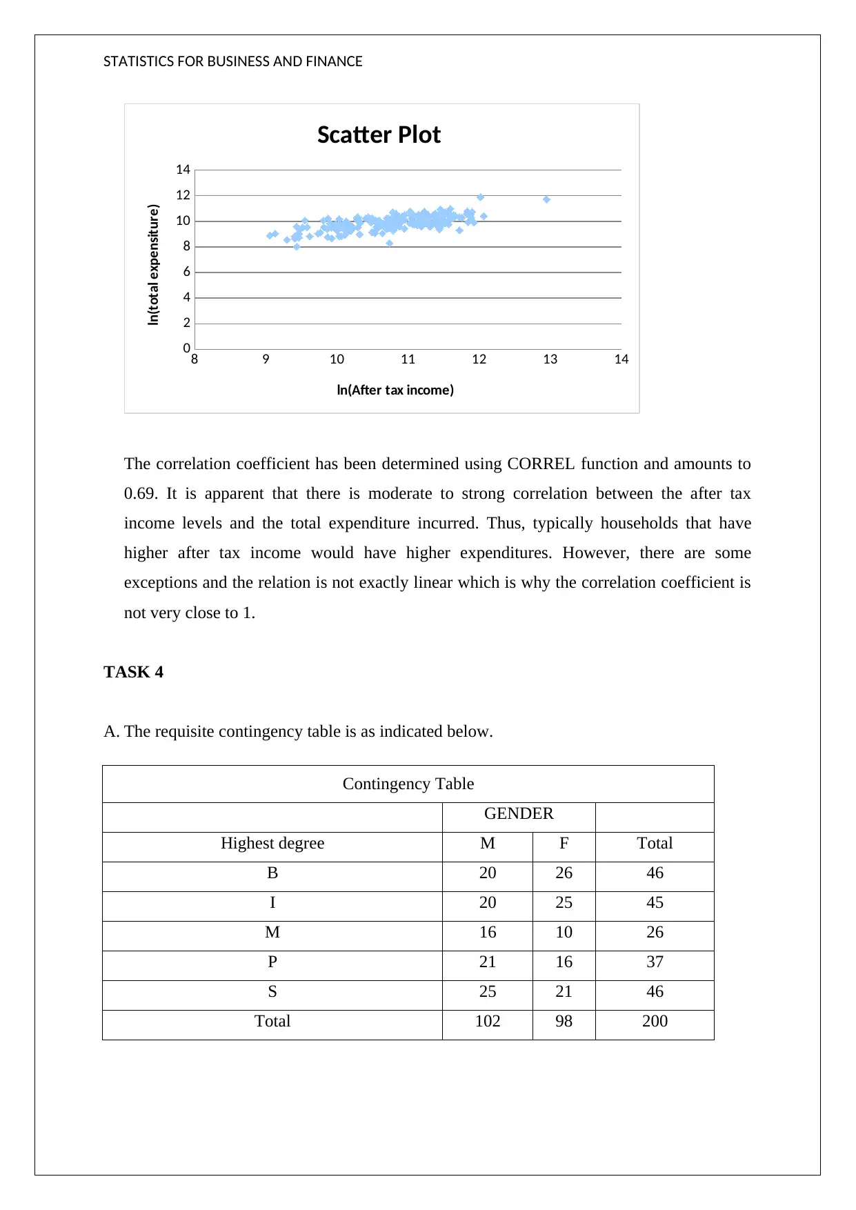
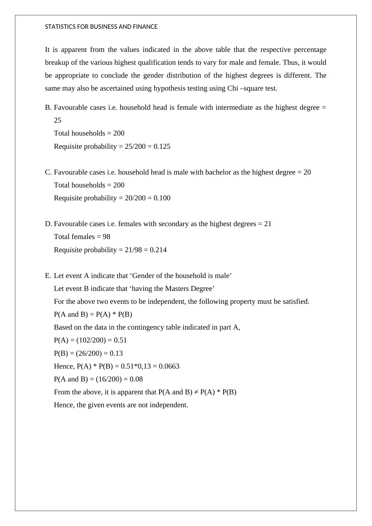
This statistics assignment analyzes a household survey dataset, encompassing various statistical techniques. Task 1 involves descriptive statistics, including measures of central tendency, variability (coefficient of variation), and the identification of non-normality through skewness and kurtosis, along with box plots. Task 2 focuses on frequency distribution for utilities expenditure, calculating probabilities and creating a histogram to assess distribution normality. Task 3 examines income disparity using percentiles, analyzes homeownership, calculates probabilities for family size, and explores the correlation between income and expenditure using a scatter plot and correlation coefficient. Task 4 utilizes a contingency table to analyze the relationship between gender and highest degree, calculating probabilities and determining the independence of events. The assignment demonstrates a comprehensive understanding of statistical methods applied to real-world survey data.

STATISTICS FOR BUSINESS AND FINANCE
HOUSEHOLD SURVEY
STUDENT ID:
[Pick the date]

STATISTICS FOR BUSINESS AND FINANCE
Task 1
A. A random sample of 200 samples has been drawn which is reflected in the attached excel
sheet. The sample method which has been used in random sampling as each of the entries
has equal change of being selected. This does not seem to be the most suitable method as a
stratified sampling would have been more suitable as it would have ensured that the
various key classifications would be represented in the same proportion as in the
population.
B. The required descriptive statistics for the desired variables coupled with the whisker and
box-plot has been represented in the attached excel sheet.
C. An appropriate measure of variability for the four variables would be coefficient of
variation which has been indicated below.
Particulars CoV
Alcohol 1.26
Meals 1.42
Fuel 1.02
Phone 0.94
It is apparent that minimum variation is witnessed for phone expenses while maximum
variation is expressed for meals. The coefficient of variation is the most suitable as it tends
to enhance comparison between the variation figures as each is computed with respect to
unit mean.
D. For all the given variables, since the measures of central tendency I.e. mean, median and
mode are not equal, hence the given distributions are not normal. This is also apparent
from the presence of skew and kurtosis value which is different from 3. For all the
variables, there is a high degree of positive skew or rightward skew which may be
attributed due to presence on outliers on the higher end. This may be due to some ultra –
rich households which would tend to have high spending on these items. Further, a high
kurtosis value would also impact the peak for these variables.

STATISTICS FOR BUSINESS AND FINANCE
Task 2
A. The requisite frequency distribution with regards to utilities expenditure has been drawn
using Excel and the result is as indicated below.
Frequency Distribution
Class Frequency
0 - 400 19
400 - 800 45
800 -1200 59
1200 -1600 33
1600 -2000 22
2000 -2400 6
2400-2800 7
2800-3200 3
More than 3200 6
Total 200
B. Based on the above frequency distribution table, the requisite percentage of households
can be computed.
1) Favourable cases = 19+45+59 = 134
Requisite probability = 123/200 = 0.615 or 61.5% of the households
2) Favourable cases = 33+22+6= 61
Requisite probability = 61/200 = 0.305 or 30.5% of the households
3) Favourable cases = 7+3+6= 16
Requisite probability = 16/200 = 0.08 or 8% of the households
C. The requisite histogram with regards to utilities expenditure has been drawn using Excel
and is as indicated below.

STATISTICS FOR BUSINESS AND FINANCE
0 - 400 400 -
800 800 -
1200 1200 -
1600 1600 -
2000 2000 -
2400 2400-
2800 2800-
3200 More
than
3200
0
10
20
30
40
50
60
70
Histogram
Expenditure on utility ($)
Frequency
The utility expenditure is not normally distributed as there is presence of positive skew which
is apparent from the above histogram. For a normal distribution, the amount of skew present
should be zero which is not the case here.
Task 3
A. The top 10% value for annual after tax income is $ 106,248.2 while the bottom 10% value
for annual after tax income is $19,098.8. These two values indicate difference between the
richest and poorest sections of the society and thereby indicate the disparity in income
levels.
B. The mean of the ownhouse variable comes out to be 0.75 which indicates that 75% of the
sample houses are used by the owners while 25% have been rented to tenants.
C. Based, on the excel output, favourable cases i.e. households with family size of 5 = 9
Total households = 200
Hence, requisite probability = 9/200 = 0.045
D. The requisite scatter plot has been generated using excel and the output is attached below.

STATISTICS FOR BUSINESS AND FINANCE
8 9 10 11 12 13 14
0
2
4
6
8
10
12
14
Scatter Plot
ln(After tax income)
ln(total expensiture)
The correlation coefficient has been determined using CORREL function and amounts to
0.69. It is apparent that there is moderate to strong correlation between the after tax
income levels and the total expenditure incurred. Thus, typically households that have
higher after tax income would have higher expenditures. However, there are some
exceptions and the relation is not exactly linear which is why the correlation coefficient is
not very close to 1.
TASK 4
A. The requisite contingency table is as indicated below.
Contingency Table
GENDER
Highest degree M F Total
B 20 26 46
I 20 25 45
M 16 10 26
P 21 16 37
S 25 21 46
Total 102 98 200

STATISTICS FOR BUSINESS AND FINANCE
It is apparent from the values indicated in the above table that the respective percentage
breakup of the various highest qualification tends to vary for male and female. Thus, it would
be appropriate to conclude the gender distribution of the highest degrees is different. The
same may also be ascertained using hypothesis testing using Chi –square test.
B. Favourable cases i.e. household head is female with intermediate as the highest degree =
25
Total households = 200
Requisite probability = 25/200 = 0.125
C. Favourable cases i.e. household head is male with bachelor as the highest degree = 20
Total households = 200
Requisite probability = 20/200 = 0.100
D. Favourable cases i.e. females with secondary as the highest degrees = 21
Total females = 98
Requisite probability = 21/98 = 0.214
E. Let event A indicate that ‘Gender of the household is male’
Let event B indicate that ‘having the Masters Degree’
For the above two events to be independent, the following property must be satisfied.
P(A and B) = P(A) * P(B)
Based on the data in the contingency table indicated in part A,
P(A) = (102/200) = 0.51
P(B) = (26/200) = 0.13
Hence, P(A) * P(B) = 0.51*0,13 = 0.0663
P(A and B) = (16/200) = 0.08
From the above, it is apparent that P(A and B) ≠ P(A) * P(B)
Hence, the given events are not independent.