Statistics Assignment: Statistical Tests, Interpretation, and Analysis
VerifiedAdded on 2023/04/22
|12
|2065
|109
Homework Assignment
AI Summary
This statistics assignment provides comprehensive solutions to various statistical tests and analyses. The assignment covers a range of topics including ANOVA, Chi-square tests, independent samples t-tests, correlation, and regression analysis. The solutions include detailed calculations, hypothesis formulations, and interpretations of results in APA format. The assignment explores the characteristics of correlations, including the interpretation of R-squared values, and provides guidance on formulating regression equations. Additionally, the document analyzes the relationship between different variables, such as milk type and baby weight, gender and school uniform preference, and smoking habits. The assignment also covers the calculation of mean, median, and standard deviation, and includes graphical representations of the data. Overall, the assignment provides a thorough understanding of various statistical concepts and their practical applications.

Statistics
Student Name:
Instructor Name:
Course Number:
14 April 2019
Student Name:
Instructor Name:
Course Number:
14 April 2019
Paraphrase This Document
Need a fresh take? Get an instant paraphrase of this document with our AI Paraphraser
Question 1:
a) Apply the information provided in the above SPSS/PSPP output to derive the value of the
following. Show your calculations clearly and round your answers to the nearest 2
decimal places.
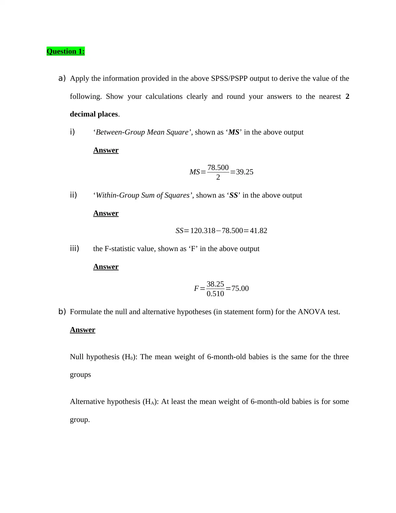
i) ‘Between-Group Mean Square’, shown as ‘MS’ in the above output
Answer
MS= 78.500
2 =39.25
ii) ‘Within-Group Sum of Squares’, shown as ‘SS’ in the above output
Answer
SS=120.318−78.500=41.82
iii) the F-statistic value, shown as ‘F’ in the above output
Answer
F= 38.25
0.510 =75.00
b) Formulate the null and alternative hypotheses (in statement form) for the ANOVA test.
Answer
Null hypothesis (H0): The mean weight of 6-month-old babies is the same for the three
groups
Alternative hypothesis (HA): At least the mean weight of 6-month-old babies is for some
group.
a) Apply the information provided in the above SPSS/PSPP output to derive the value of the
following. Show your calculations clearly and round your answers to the nearest 2
decimal places.
i) ‘Between-Group Mean Square’, shown as ‘MS’ in the above output
Answer
MS= 78.500
2 =39.25
ii) ‘Within-Group Sum of Squares’, shown as ‘SS’ in the above output
Answer
SS=120.318−78.500=41.82
iii) the F-statistic value, shown as ‘F’ in the above output
Answer
F= 38.25
0.510 =75.00
b) Formulate the null and alternative hypotheses (in statement form) for the ANOVA test.
Answer
Null hypothesis (H0): The mean weight of 6-month-old babies is the same for the three
groups
Alternative hypothesis (HA): At least the mean weight of 6-month-old babies is for some
group.
c) At α = .05, test the hypothesis that you have formulated in (b). Analyse the results of the
test and report your findings in APA format (round your answers to the nearest 2 decimal
places).
Answer
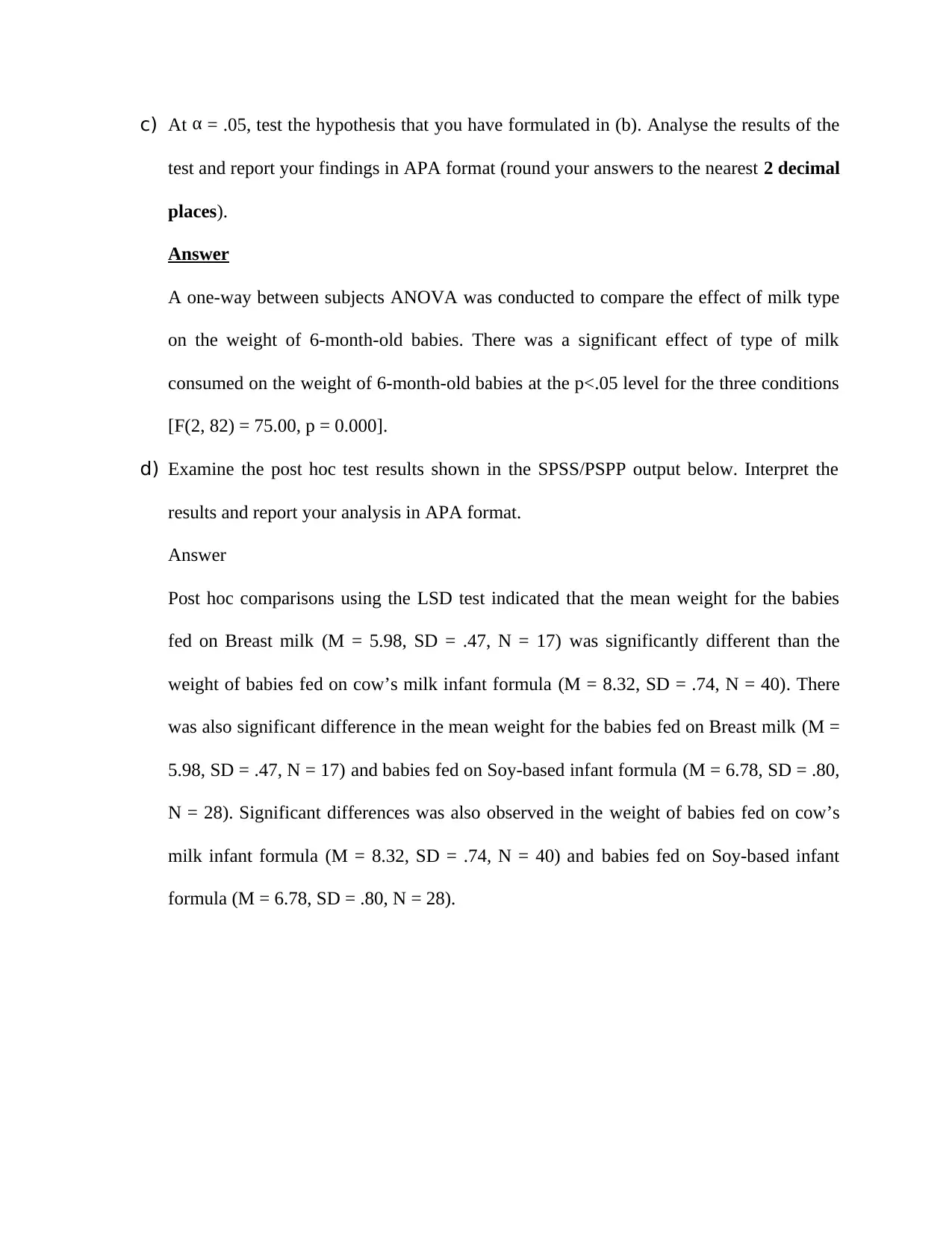
A one-way between subjects ANOVA was conducted to compare the effect of milk type
on the weight of 6-month-old babies. There was a significant effect of type of milk
consumed on the weight of 6-month-old babies at the p<.05 level for the three conditions
[F(2, 82) = 75.00, p = 0.000].
d) Examine the post hoc test results shown in the SPSS/PSPP output below. Interpret the
results and report your analysis in APA format.
Answer
Post hoc comparisons using the LSD test indicated that the mean weight for the babies
fed on Breast milk (M = 5.98, SD = .47, N = 17) was significantly different than the
weight of babies fed on cow’s milk infant formula (M = 8.32, SD = .74, N = 40). There
was also significant difference in the mean weight for the babies fed on Breast milk (M =
5.98, SD = .47, N = 17) and babies fed on Soy-based infant formula (M = 6.78, SD = .80,
N = 28). Significant differences was also observed in the weight of babies fed on cow’s
milk infant formula (M = 8.32, SD = .74, N = 40) and babies fed on Soy-based infant
formula (M = 6.78, SD = .80, N = 28).
test and report your findings in APA format (round your answers to the nearest 2 decimal
places).
Answer
A one-way between subjects ANOVA was conducted to compare the effect of milk type
on the weight of 6-month-old babies. There was a significant effect of type of milk
consumed on the weight of 6-month-old babies at the p<.05 level for the three conditions
[F(2, 82) = 75.00, p = 0.000].
d) Examine the post hoc test results shown in the SPSS/PSPP output below. Interpret the
results and report your analysis in APA format.
Answer
Post hoc comparisons using the LSD test indicated that the mean weight for the babies
fed on Breast milk (M = 5.98, SD = .47, N = 17) was significantly different than the
weight of babies fed on cow’s milk infant formula (M = 8.32, SD = .74, N = 40). There
was also significant difference in the mean weight for the babies fed on Breast milk (M =
5.98, SD = .47, N = 17) and babies fed on Soy-based infant formula (M = 6.78, SD = .80,
N = 28). Significant differences was also observed in the weight of babies fed on cow’s
milk infant formula (M = 8.32, SD = .74, N = 40) and babies fed on Soy-based infant
formula (M = 6.78, SD = .80, N = 28).
⊘ This is a preview!⊘
Do you want full access?
Subscribe today to unlock all pages.
Trusted by 1+ million students worldwide
Question 2:
a) Formulation of the hypothesis
Answer
Null hypothesis (H0): The gender differences in the preference of school uniform designs
are not random
Alternative hypothesis (HA): The gender differences in the preference of school uniform
designs are random.
b) Calculating the chi-square statistic χ2
Answer
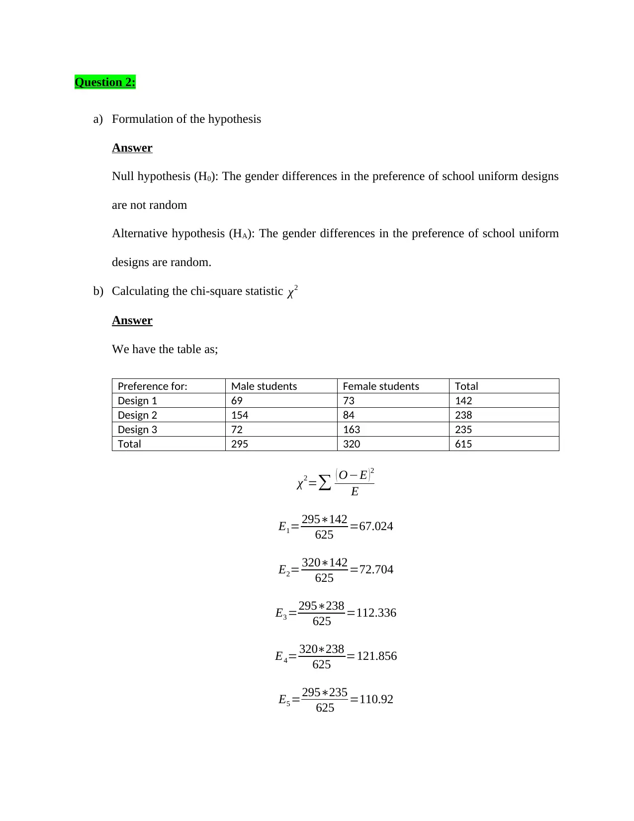
We have the table as;
Preference for: Male students Female students Total
Design 1 69 73 142
Design 2 154 84 238
Design 3 72 163 235
Total 295 320 615
χ2=∑ ( O−E )2
E
E1= 295∗142
625 =67.024
E2= 320∗142
625 =72.704
E3 =295∗238
625 =112.336
E4= 320∗238
625 =121.856
E5 =295∗235
625 =110.92
a) Formulation of the hypothesis
Answer
Null hypothesis (H0): The gender differences in the preference of school uniform designs
are not random
Alternative hypothesis (HA): The gender differences in the preference of school uniform
designs are random.
b) Calculating the chi-square statistic χ2
Answer
We have the table as;
Preference for: Male students Female students Total
Design 1 69 73 142
Design 2 154 84 238
Design 3 72 163 235
Total 295 320 615
χ2=∑ ( O−E )2
E
E1= 295∗142
625 =67.024
E2= 320∗142
625 =72.704
E3 =295∗238
625 =112.336
E4= 320∗238
625 =121.856
E5 =295∗235
625 =110.92
Paraphrase This Document
Need a fresh take? Get an instant paraphrase of this document with our AI Paraphraser
E6 =320∗235
625 =120.32
χ2=∑ ( O−E ) 2
E = ( 69−67.024 )2
67.024 + ( 73−72.704 )2
72.704 + ( 154−112.336 ) 2
112.336 + ( 84−121.856 ) 2
121.856 + ( 72−110.92 ) 2
110.92 + ( 163
1
Effect size computation
φ= √ χ 2
n = √ 56.07
615 = √ 0.0912=0.30
c) Reporting results in APA
Answer
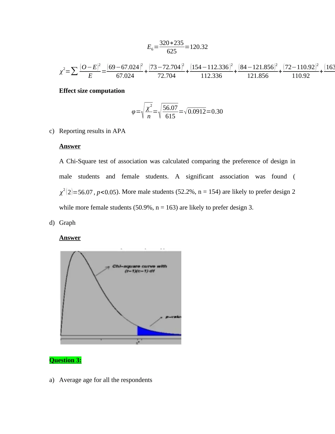
A Chi-Square test of association was calculated comparing the preference of design in
male students and female students. A significant association was found (
χ2 ( 2 )=56.07 , p<0.05). More male students (52.2%, n = 154) are likely to prefer design 2
while more female students (50.9%, n = 163) are likely to prefer design 3.
d) Graph
Answer
Question 3:
a) Average age for all the respondents
625 =120.32
χ2=∑ ( O−E ) 2
E = ( 69−67.024 )2
67.024 + ( 73−72.704 )2
72.704 + ( 154−112.336 ) 2
112.336 + ( 84−121.856 ) 2
121.856 + ( 72−110.92 ) 2
110.92 + ( 163
1
Effect size computation
φ= √ χ 2
n = √ 56.07
615 = √ 0.0912=0.30
c) Reporting results in APA
Answer
A Chi-Square test of association was calculated comparing the preference of design in
male students and female students. A significant association was found (
χ2 ( 2 )=56.07 , p<0.05). More male students (52.2%, n = 154) are likely to prefer design 2
while more female students (50.9%, n = 163) are likely to prefer design 3.
d) Graph
Answer
Question 3:
a) Average age for all the respondents
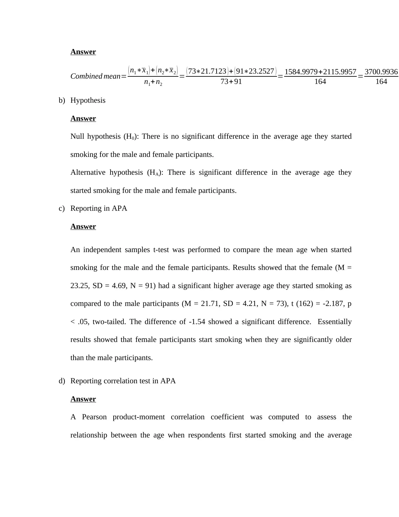
Answer
Combined mean= ( n1∗x1 ) + ( n2∗x2 )
n1+n2
= ( 73∗21.7123 )+ ( 91∗23.2527 )
73+ 91 = 1584.9979+2115.9957
164 = 3700.9936
164 =
b) Hypothesis
Answer
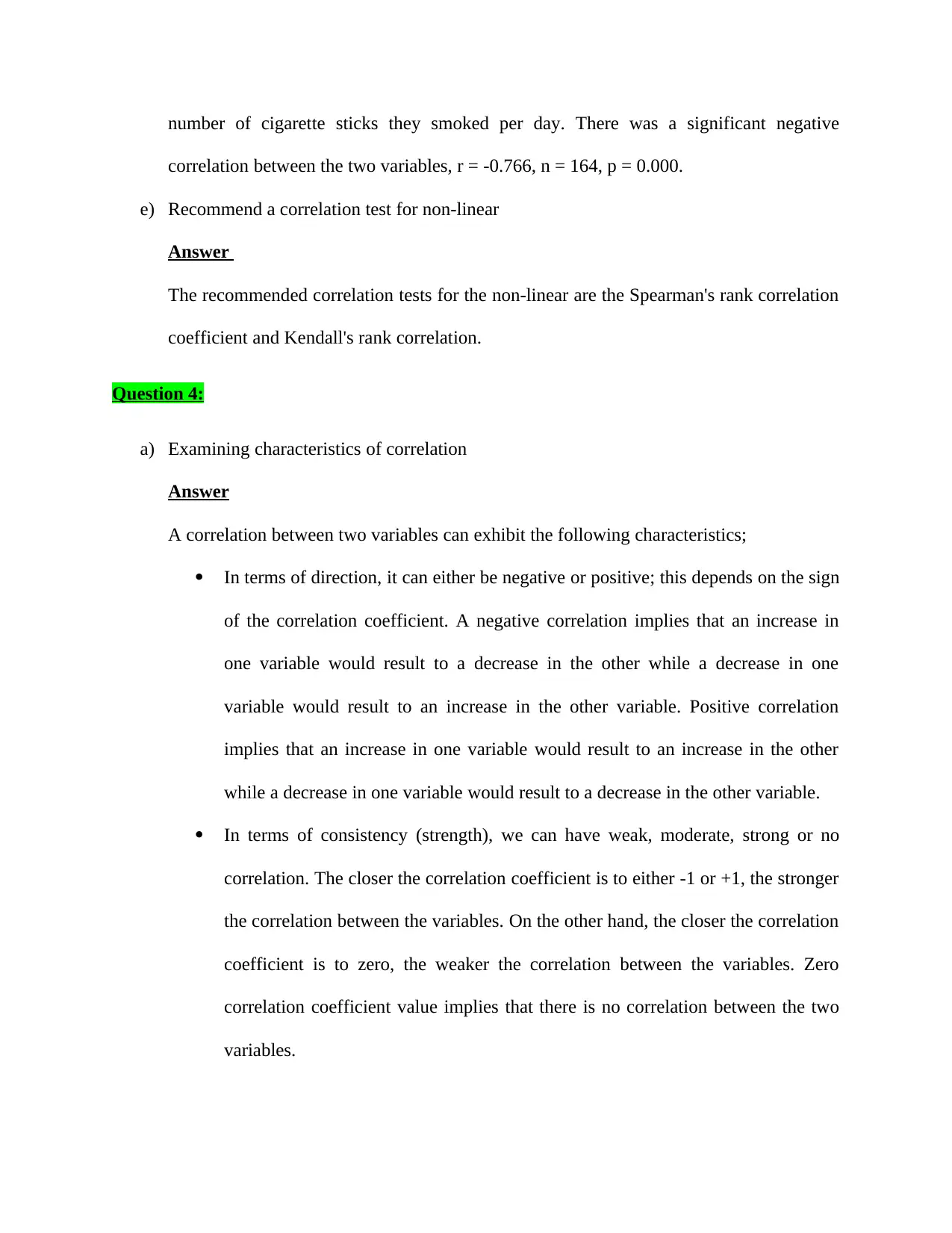
Null hypothesis (H0): There is no significant difference in the average age they started
smoking for the male and female participants.
Alternative hypothesis (HA): There is significant difference in the average age they
started smoking for the male and female participants.
c) Reporting in APA
Answer
An independent samples t-test was performed to compare the mean age when started
smoking for the male and the female participants. Results showed that the female (M =
23.25, SD = 4.69, N = 91) had a significant higher average age they started smoking as
compared to the male participants (M = 21.71, SD = 4.21, N = 73), t (162) = -2.187, p
< .05, two-tailed. The difference of -1.54 showed a significant difference. Essentially
results showed that female participants start smoking when they are significantly older
than the male participants.
d) Reporting correlation test in APA
Answer
A Pearson product-moment correlation coefficient was computed to assess the
relationship between the age when respondents first started smoking and the average
Combined mean= ( n1∗x1 ) + ( n2∗x2 )
n1+n2
= ( 73∗21.7123 )+ ( 91∗23.2527 )
73+ 91 = 1584.9979+2115.9957
164 = 3700.9936
164 =
b) Hypothesis
Answer
Null hypothesis (H0): There is no significant difference in the average age they started
smoking for the male and female participants.
Alternative hypothesis (HA): There is significant difference in the average age they
started smoking for the male and female participants.
c) Reporting in APA
Answer
An independent samples t-test was performed to compare the mean age when started
smoking for the male and the female participants. Results showed that the female (M =
23.25, SD = 4.69, N = 91) had a significant higher average age they started smoking as
compared to the male participants (M = 21.71, SD = 4.21, N = 73), t (162) = -2.187, p
< .05, two-tailed. The difference of -1.54 showed a significant difference. Essentially
results showed that female participants start smoking when they are significantly older
than the male participants.
d) Reporting correlation test in APA
Answer
A Pearson product-moment correlation coefficient was computed to assess the
relationship between the age when respondents first started smoking and the average
⊘ This is a preview!⊘
Do you want full access?
Subscribe today to unlock all pages.
Trusted by 1+ million students worldwide
number of cigarette sticks they smoked per day. There was a significant negative
correlation between the two variables, r = -0.766, n = 164, p = 0.000.
e) Recommend a correlation test for non-linear
Answer
The recommended correlation tests for the non-linear are the Spearman's rank correlation
coefficient and Kendall's rank correlation.
Question 4:
a) Examining characteristics of correlation
Answer
A correlation between two variables can exhibit the following characteristics;
In terms of direction, it can either be negative or positive; this depends on the sign
of the correlation coefficient. A negative correlation implies that an increase in
one variable would result to a decrease in the other while a decrease in one
variable would result to an increase in the other variable. Positive correlation
implies that an increase in one variable would result to an increase in the other
while a decrease in one variable would result to a decrease in the other variable.
In terms of consistency (strength), we can have weak, moderate, strong or no
correlation. The closer the correlation coefficient is to either -1 or +1, the stronger
the correlation between the variables. On the other hand, the closer the correlation
coefficient is to zero, the weaker the correlation between the variables. Zero
correlation coefficient value implies that there is no correlation between the two
variables.
Paraphrase This Document
Need a fresh take? Get an instant paraphrase of this document with our AI Paraphraser
It is wrong to assume causality in correlation analysis because correlation does not
necessarily imply causation. For example, there could be correlation between the number
ice creams sold and the number of homicides. However, it does not mean that ice cream
consumption causes homicide.
b) Correlation between the percentage of body fat and body mass index (BMI)
i) Interpretation of R2 value
Answer
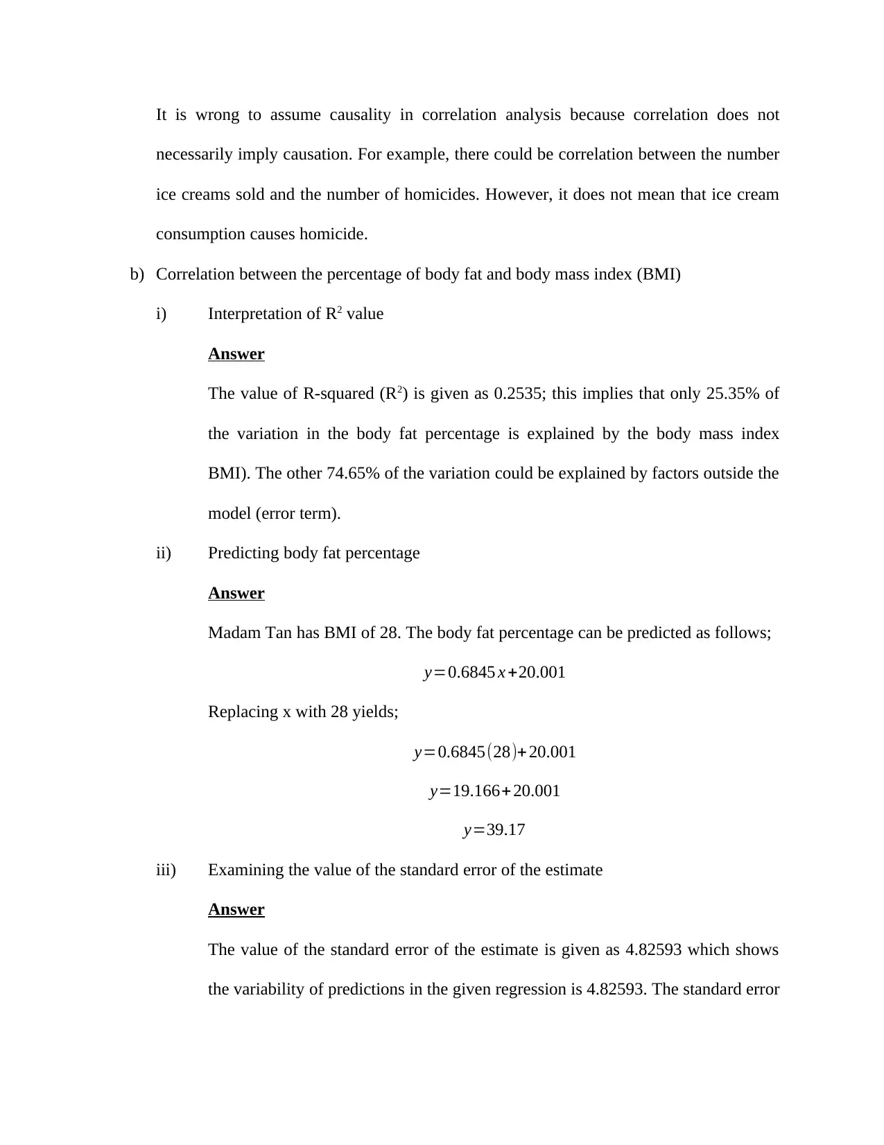
The value of R-squared (R2) is given as 0.2535; this implies that only 25.35% of
the variation in the body fat percentage is explained by the body mass index
BMI). The other 74.65% of the variation could be explained by factors outside the
model (error term).
ii) Predicting body fat percentage
Answer
Madam Tan has BMI of 28. The body fat percentage can be predicted as follows;
y=0.6845 x +20.001
Replacing x with 28 yields;
y=0.6845(28)+ 20.001
y=19.166+ 20.001
y=39.17
iii) Examining the value of the standard error of the estimate
Answer
The value of the standard error of the estimate is given as 4.82593 which shows
the variability of predictions in the given regression is 4.82593. The standard error
necessarily imply causation. For example, there could be correlation between the number
ice creams sold and the number of homicides. However, it does not mean that ice cream
consumption causes homicide.
b) Correlation between the percentage of body fat and body mass index (BMI)
i) Interpretation of R2 value
Answer
The value of R-squared (R2) is given as 0.2535; this implies that only 25.35% of
the variation in the body fat percentage is explained by the body mass index
BMI). The other 74.65% of the variation could be explained by factors outside the
model (error term).
ii) Predicting body fat percentage
Answer
Madam Tan has BMI of 28. The body fat percentage can be predicted as follows;
y=0.6845 x +20.001
Replacing x with 28 yields;
y=0.6845(28)+ 20.001
y=19.166+ 20.001
y=39.17
iii) Examining the value of the standard error of the estimate
Answer
The value of the standard error of the estimate is given as 4.82593 which shows
the variability of predictions in the given regression is 4.82593. The standard error
of the estimate is important in the regression as it shows how close the
observations are to the fitted regression line.
Question 5:
a) Determining mean and median and explaining the distribution
Answer
non-regular
exercisers
regular
exercisers
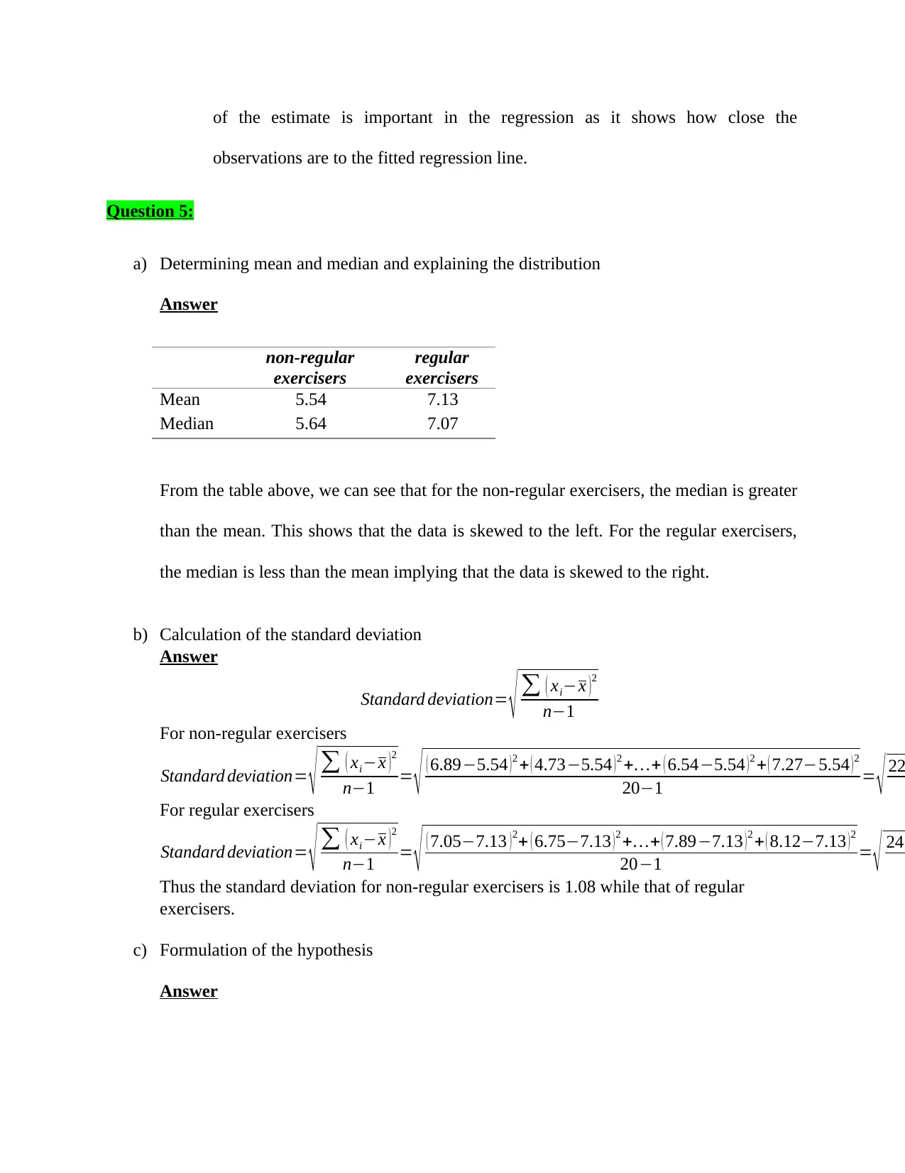
Mean 5.54 7.13
Median 5.64 7.07
From the table above, we can see that for the non-regular exercisers, the median is greater
than the mean. This shows that the data is skewed to the left. For the regular exercisers,
the median is less than the mean implying that the data is skewed to the right.
b) Calculation of the standard deviation
Answer
Standard deviation= √ ∑ ( xi−x ) 2
n−1
For non-regular exercisers
Standard deviation= √ ∑ ( xi−x ) 2
n−1 = √ ( 6.89−5.54 ) 2 + ( 4.73−5.54 ) 2 +…+ ( 6.54−5.54 ) 2 + ( 7.27−5.54 ) 2
20−1 = √ 22
For regular exercisers
Standard deviation= √ ∑ ( xi−x ) 2
n−1 = √ ( 7.05−7.13 ) 2+ ( 6.75−7.13 ) 2 +…+ ( 7.89−7.13 ) 2 + ( 8.12−7.13 ) 2
20−1 = √ 24.
Thus the standard deviation for non-regular exercisers is 1.08 while that of regular
exercisers.
c) Formulation of the hypothesis
Answer
observations are to the fitted regression line.
Question 5:
a) Determining mean and median and explaining the distribution
Answer
non-regular
exercisers
regular
exercisers
Mean 5.54 7.13
Median 5.64 7.07
From the table above, we can see that for the non-regular exercisers, the median is greater
than the mean. This shows that the data is skewed to the left. For the regular exercisers,
the median is less than the mean implying that the data is skewed to the right.
b) Calculation of the standard deviation
Answer
Standard deviation= √ ∑ ( xi−x ) 2
n−1
For non-regular exercisers
Standard deviation= √ ∑ ( xi−x ) 2
n−1 = √ ( 6.89−5.54 ) 2 + ( 4.73−5.54 ) 2 +…+ ( 6.54−5.54 ) 2 + ( 7.27−5.54 ) 2
20−1 = √ 22
For regular exercisers
Standard deviation= √ ∑ ( xi−x ) 2
n−1 = √ ( 7.05−7.13 ) 2+ ( 6.75−7.13 ) 2 +…+ ( 7.89−7.13 ) 2 + ( 8.12−7.13 ) 2
20−1 = √ 24.
Thus the standard deviation for non-regular exercisers is 1.08 while that of regular
exercisers.
c) Formulation of the hypothesis
Answer
⊘ This is a preview!⊘
Do you want full access?
Subscribe today to unlock all pages.
Trusted by 1+ million students worldwide
Null hypothesis (H0): There is no significant difference in the average physical well-
being score for the non-regular exercisers and regular exercisers.
Alternative hypothesis (HA): There is significant difference in the average physical well-
being score for the non-regular exercisers and regular exercisers.
d) Reporting in APA
Answer
An independent samples t-test was performed to compare the average physical well-being
score for the non-regular exercisers and regular exercisers. Results showed that there is
significant difference in the average physical well-being score for the non-regular
exercisers and regular exercisers t(38) – 4.524, p = .000. Regular exercisers on average
reported higher physical well-being score than the non-regular exercisers.
Question 6:
a) Characteristics of the correlations between the two variables
Answer
There is a strong correlation between the variables; we have been provided
with the correlation coefficient to be 0.804 which shows that the correlation is
strong since it I close to +1.
There is a positive correlation between the variables; we have been provided
with the correlation coefficient to be 0.804. The sign is positive which shows
that the correlation is positive
There is a linear correlation between the variables; the graph provided shows
the values to be in a linear form indicating that the correlation between the
variables is linear.
being score for the non-regular exercisers and regular exercisers.
Alternative hypothesis (HA): There is significant difference in the average physical well-
being score for the non-regular exercisers and regular exercisers.
d) Reporting in APA
Answer
An independent samples t-test was performed to compare the average physical well-being
score for the non-regular exercisers and regular exercisers. Results showed that there is
significant difference in the average physical well-being score for the non-regular
exercisers and regular exercisers t(38) – 4.524, p = .000. Regular exercisers on average
reported higher physical well-being score than the non-regular exercisers.
Question 6:
a) Characteristics of the correlations between the two variables
Answer
There is a strong correlation between the variables; we have been provided
with the correlation coefficient to be 0.804 which shows that the correlation is
strong since it I close to +1.
There is a positive correlation between the variables; we have been provided
with the correlation coefficient to be 0.804. The sign is positive which shows
that the correlation is positive
There is a linear correlation between the variables; the graph provided shows
the values to be in a linear form indicating that the correlation between the
variables is linear.
Paraphrase This Document
Need a fresh take? Get an instant paraphrase of this document with our AI Paraphraser
b) Analyzing and explaining the data in APA
Answer
A Pearson product-moment correlation coefficient was computed to assess the
relationship between the continuous assessment scores and the exam scores. There
was a significant positive correlation between the two variables, r = 0.804, n = 30, p =
0.000.
c) Formulating regression equation and predicting the scores
Answer
From the regression output, we can formulate the regression equation as follows;
Exam score=−28.416+1.212(CA)
Predicting X student’s CA score given that the student scored 52 in exam.
Exam score=−28.416+1.212(CA)
52=−28.416+1.212(CA)
1.212 (CA )=52+28.416
1.212 ( CA ) =80.416
CA=80.416
1.212 =66.35
So student X must have scored 66.35 in the continuous assessment (CA).
From the output, we observe the p-value for the continuous assessment to be 0.000 (a
value less than 5% level of significance), we there reject the null hypothesis and
conclude that continuous assessment is a significant predictor of exam scores.
Answer
A Pearson product-moment correlation coefficient was computed to assess the
relationship between the continuous assessment scores and the exam scores. There
was a significant positive correlation between the two variables, r = 0.804, n = 30, p =
0.000.
c) Formulating regression equation and predicting the scores
Answer
From the regression output, we can formulate the regression equation as follows;
Exam score=−28.416+1.212(CA)
Predicting X student’s CA score given that the student scored 52 in exam.
Exam score=−28.416+1.212(CA)
52=−28.416+1.212(CA)
1.212 (CA )=52+28.416
1.212 ( CA ) =80.416
CA=80.416
1.212 =66.35
So student X must have scored 66.35 in the continuous assessment (CA).
From the output, we observe the p-value for the continuous assessment to be 0.000 (a
value less than 5% level of significance), we there reject the null hypothesis and
conclude that continuous assessment is a significant predictor of exam scores.

⊘ This is a preview!⊘
Do you want full access?
Subscribe today to unlock all pages.
Trusted by 1+ million students worldwide
1 out of 12
Your All-in-One AI-Powered Toolkit for Academic Success.
+13062052269
info@desklib.com
Available 24*7 on WhatsApp / Email
![[object Object]](/_next/static/media/star-bottom.7253800d.svg)
Unlock your academic potential
Copyright © 2020–2026 A2Z Services. All Rights Reserved. Developed and managed by ZUCOL.