Statistical Methods for Business: A Management Report and Analysis

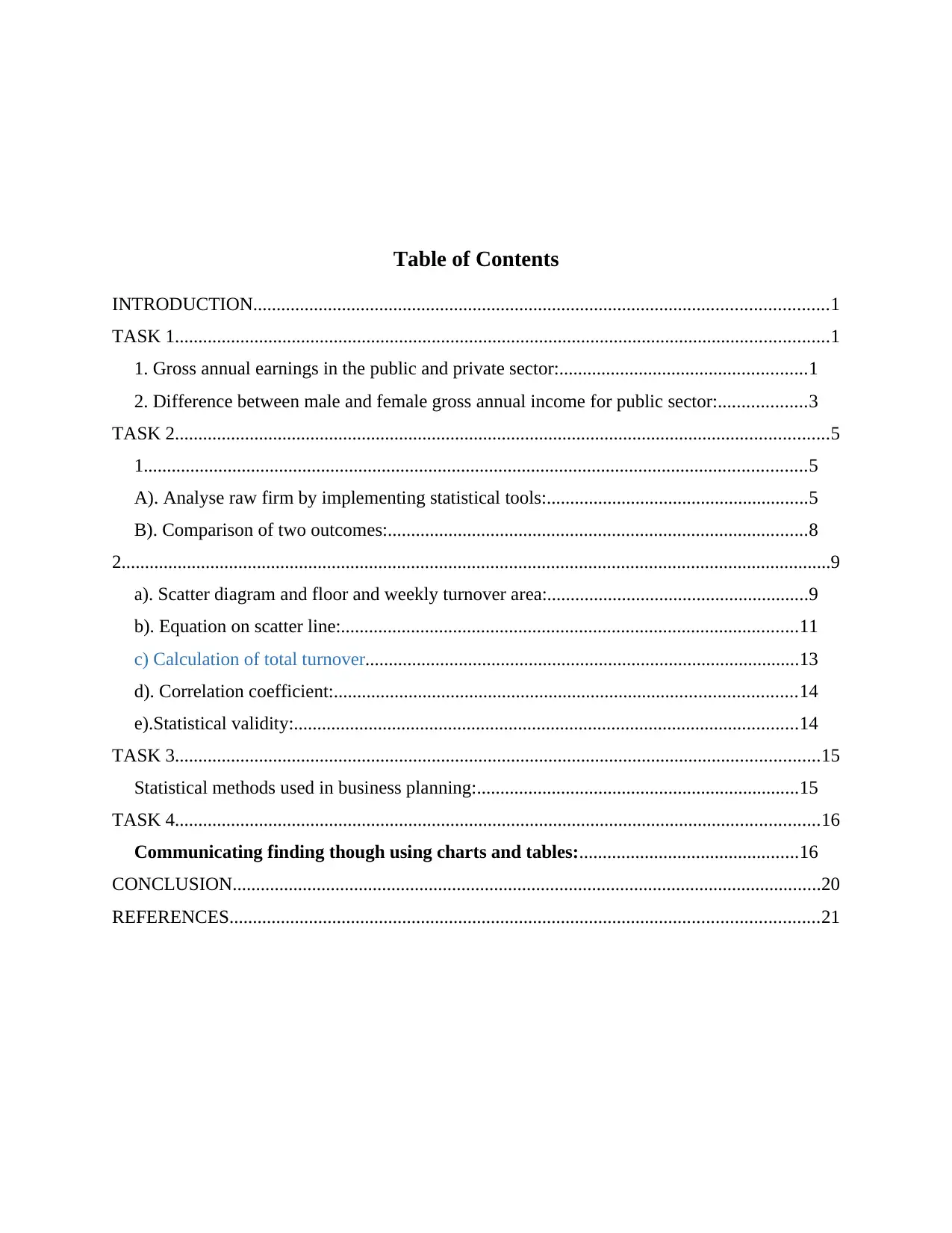
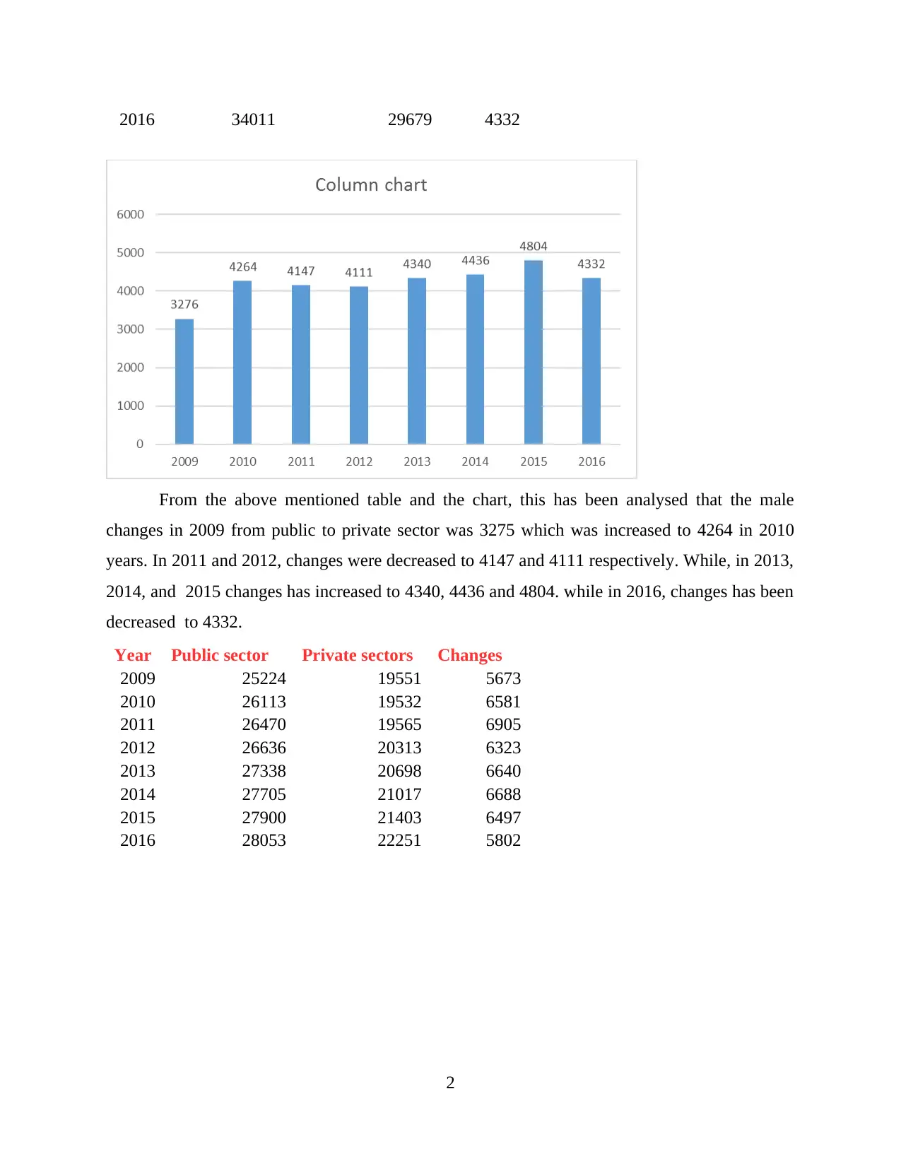
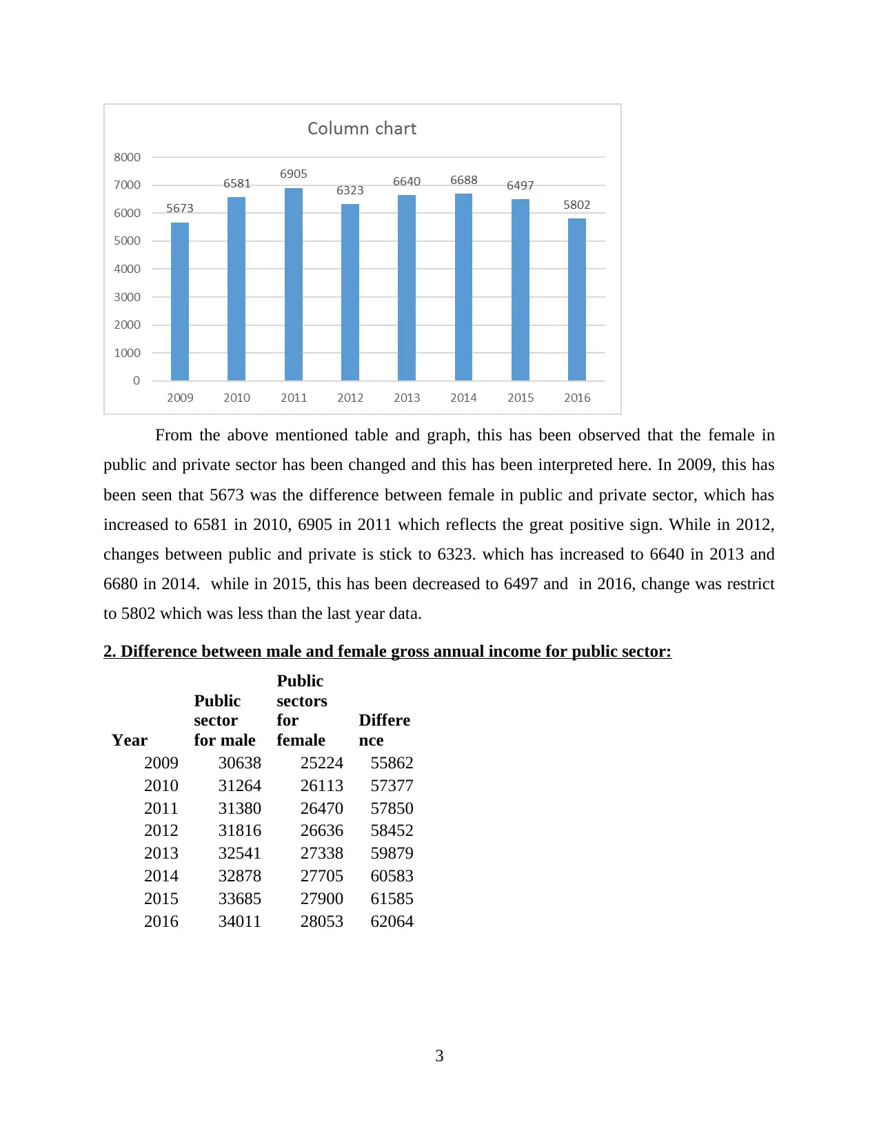
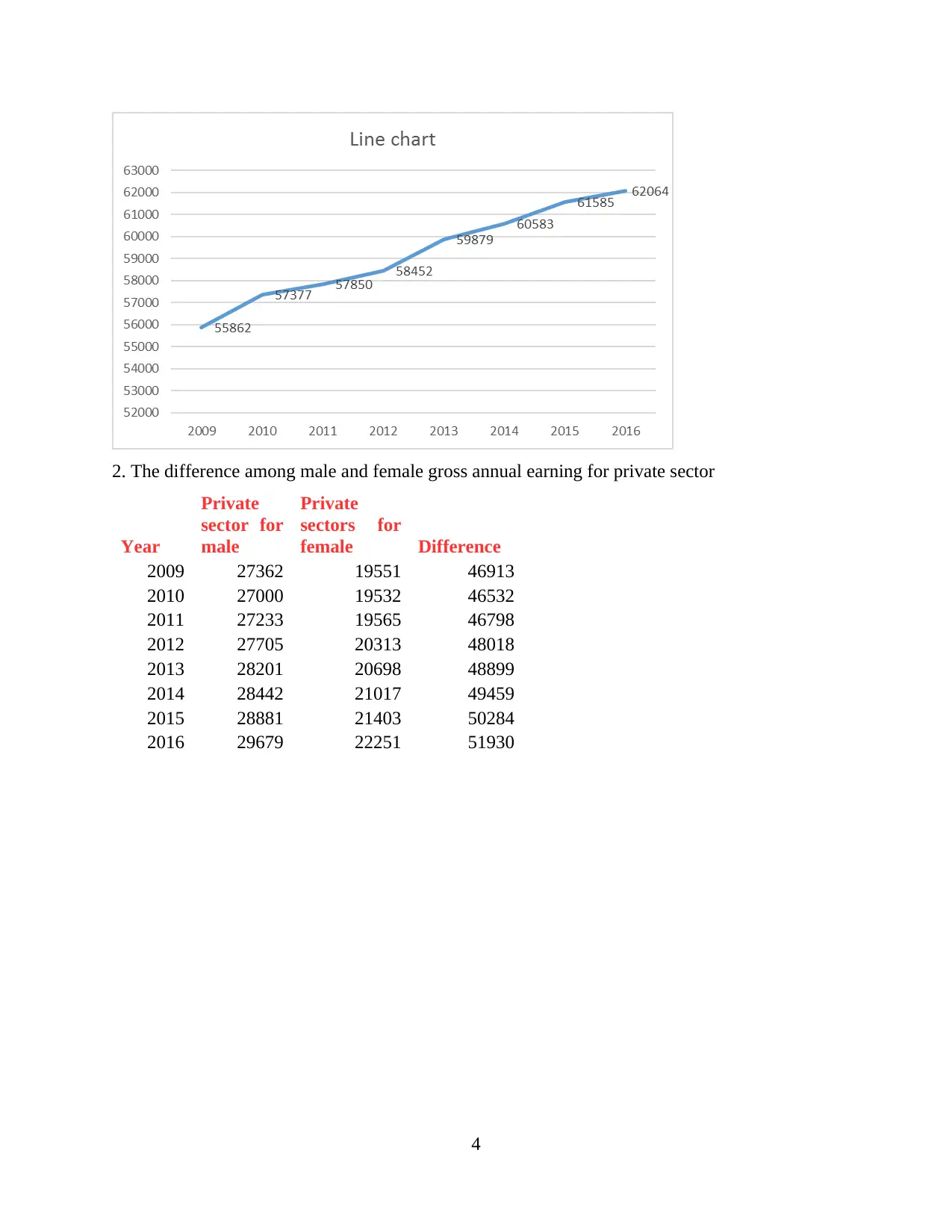
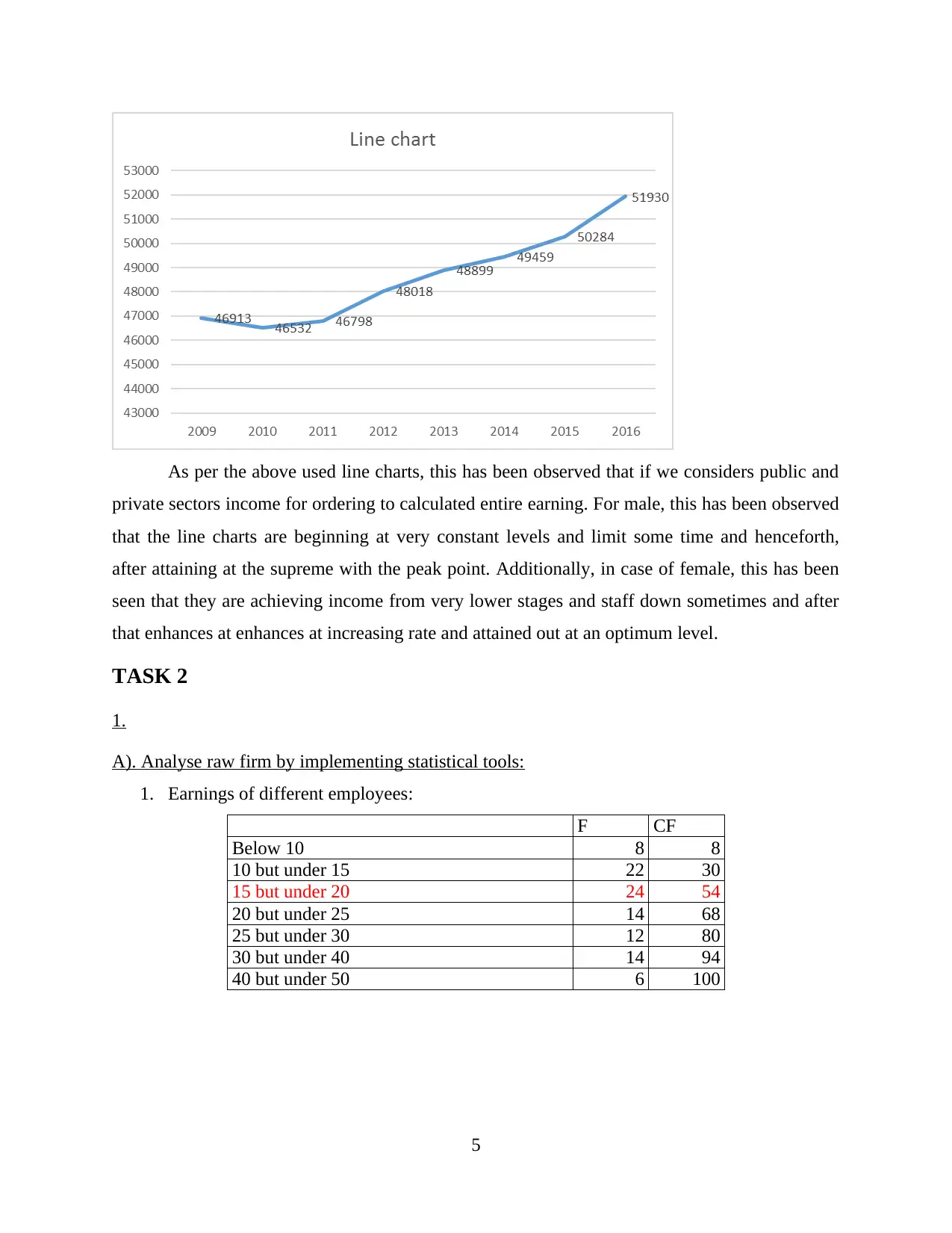
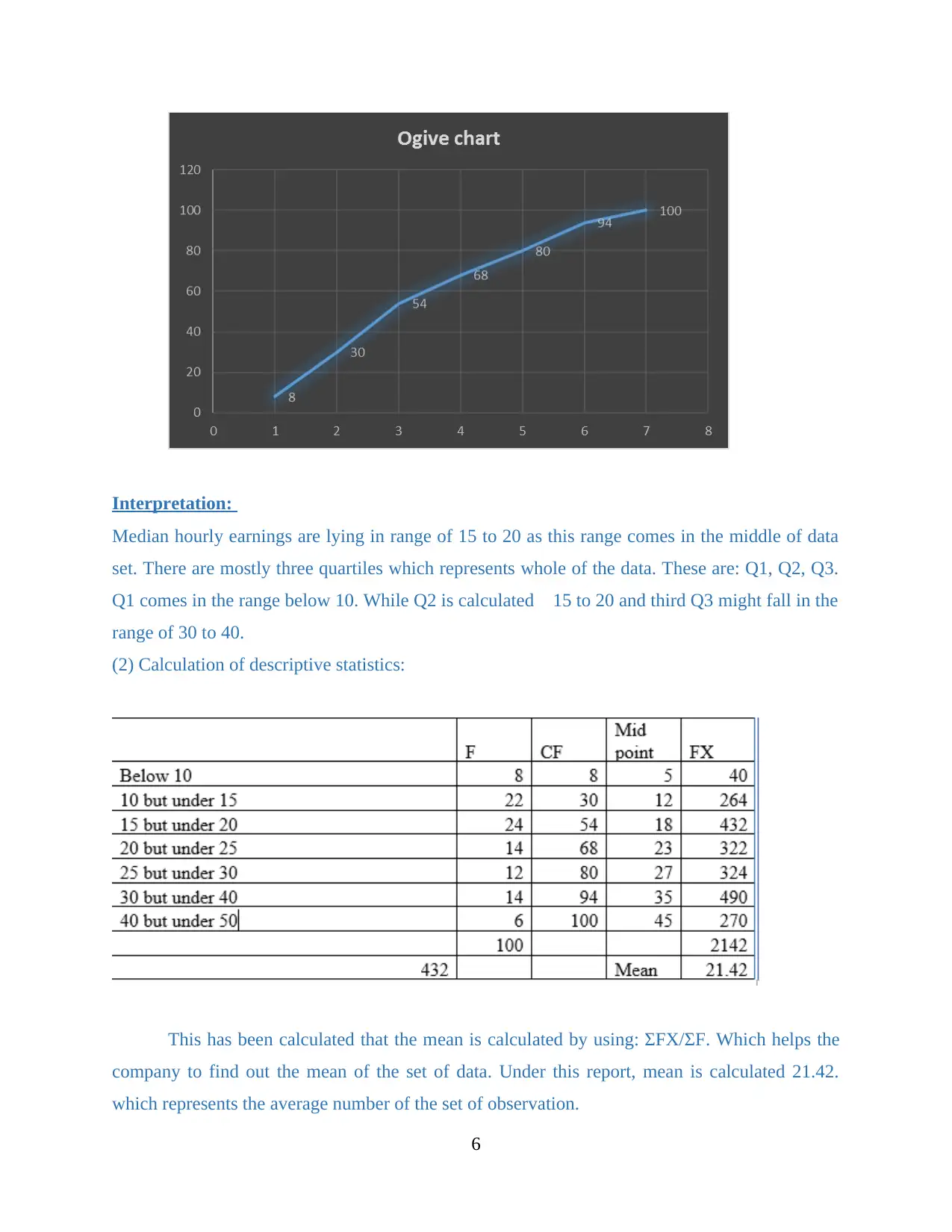
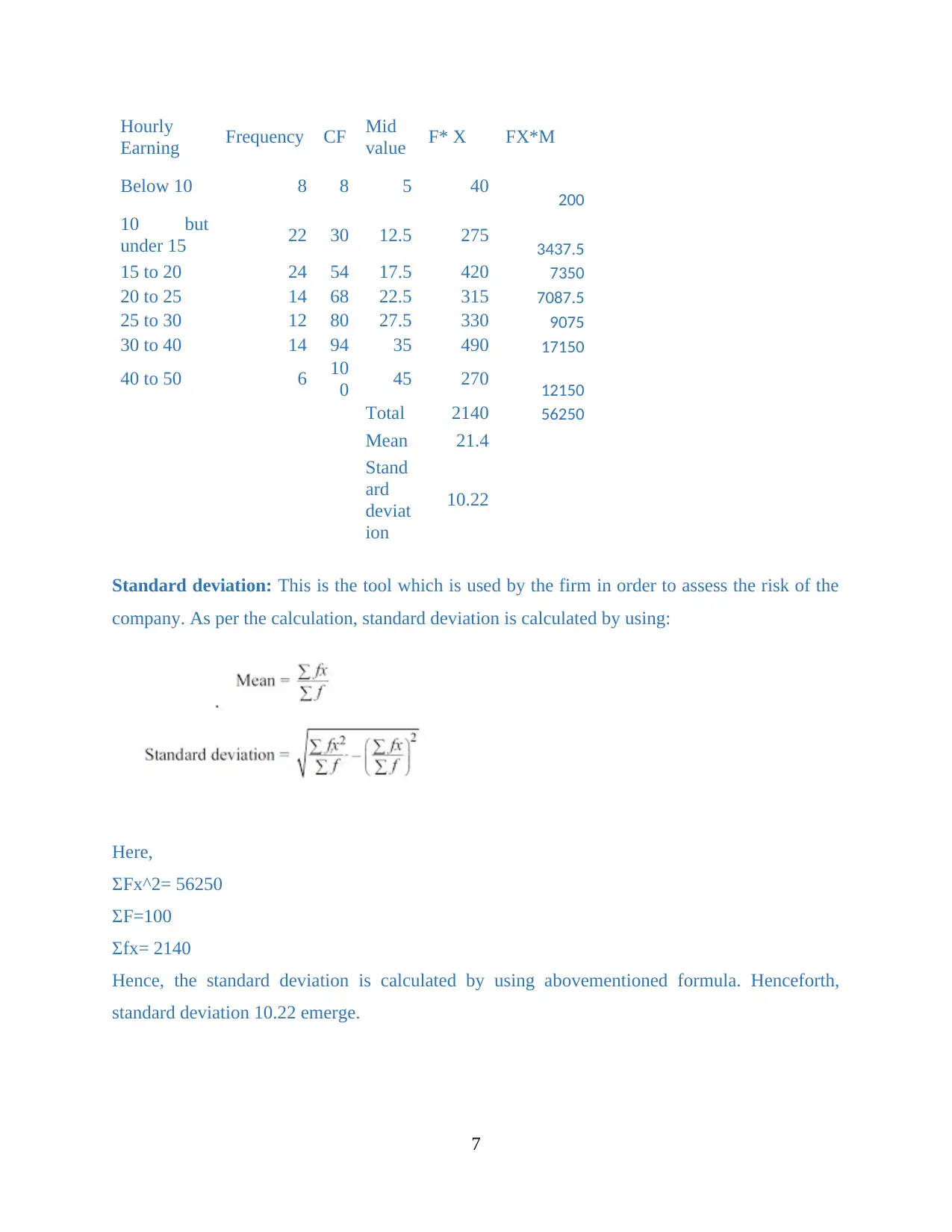
This report provides a comprehensive statistical analysis for management, covering various aspects of data analysis and business planning. The introduction highlights the crucial role of statistics in business decision-making, emphasizing the need for accurate data to assess positive outcomes. Task 1 focuses on gross annual earnings in the public and private sectors, comparing male and female incomes over several years using tables and charts. Task 2 delves into analyzing raw firm data with statistical tools, including the calculation of descriptive statistics like mean, standard deviation, median, and mode. It also compares two outcomes based on statistical data and includes a scatter diagram to analyze the relationship between outlet size and turnover, along with the calculation of the correlation coefficient. Task 3 discusses the application of statistical methods in business planning, and Task 4 focuses on communicating findings through charts and tables. The report concludes with a summary of the key findings and recommendations based on the statistical analysis.

Statistic for management

Table of Contents
INTRODUCTION...........................................................................................................................1
TASK 1............................................................................................................................................1
1. Gross annual earnings in the public and private sector:.....................................................1
2. Difference between male and female gross annual income for public sector:...................3
TASK 2............................................................................................................................................5
1..............................................................................................................................................5
A). Analyse raw firm by implementing statistical tools:........................................................5
B). Comparison of two outcomes:..........................................................................................8
2........................................................................................................................................................9
a). Scatter diagram and floor and weekly turnover area:........................................................9
b). Equation on scatter line:..................................................................................................11
c) Calculation of total turnover.............................................................................................13
d). Correlation coefficient:...................................................................................................14
e).Statistical validity:............................................................................................................14
TASK 3..........................................................................................................................................15
Statistical methods used in business planning:.....................................................................15
TASK 4..........................................................................................................................................16
Communicating finding though using charts and tables:...............................................16
CONCLUSION..............................................................................................................................20
REFERENCES..............................................................................................................................21

INTRODUCTION
Statistics plays a crucial role for business decision making. Under a competitive market
environment, a firm cannot survive merely by framing decisions based on hypothesis (Anderson
and et. al., 2014). There is a need to make accurate data that will assist for assessing the positive
conclusions from the available resources. This project consists of various task explaining various
charts and graphs related with the annual earning of male and females. Various factors which are
used in analysing the collected data. On the basis of various charts necessary recommendation
are provided under this project report.
TASK 1
1. Gross annual earnings in the public and private sector:
Each employee is striving hard to attain firms individual and group goals. In return of
their work, they are getting few annual earnings after the net profit a firm get during the year.
This is the money which is earned annually (Curtis and et. al., 2011). Gross annual income refers
to the amount of fund which an individual or employee gets in one financial year from whole
concerned resources before any taxes levied on it. While making any income tax return at the
time of accounting period, the gross annual income total is taken as the base amount with which
to run.
For assessing the whole gross annual salary, there is a need to assess the appropriate
amount of pay, multiply it with the hourly wages by the total number of hours an employee is
working in a week and thereafter, multiply it with 52 (Curtis, Kim and Yalagandula, 2011). This
will come out as the annual gross income and after that it divide it by 12 to identify monthly pay
which they are getting.
Gross annual earnings for male and female is identified. Which are as follows:
Male Gross annual earnings:
Year Public sector Private sectors Changes
2009 30638 27362 3276
2010 31264 27000 4264
2011 31380 27233 4147
2012 31816 27705 4111
2013 32541 28201 4340
2014 32878 28442 4436
2015 33685 28881 4804
1

2016 34011 29679 4332
From the above mentioned table and the chart, this has been analysed that the male
changes in 2009 from public to private sector was 3275 which was increased to 4264 in 2010
years. In 2011 and 2012, changes were decreased to 4147 and 4111 respectively. While, in 2013,
2014, and 2015 changes has increased to 4340, 4436 and 4804. while in 2016, changes has been
decreased to 4332.
Year Public sector Private sectors Changes
2009 25224 19551 5673
2010 26113 19532 6581
2011 26470 19565 6905
2012 26636 20313 6323
2013 27338 20698 6640
2014 27705 21017 6688
2015 27900 21403 6497
2016 28053 22251 5802
2

From the above mentioned table and graph, this has been observed that the female in
public and private sector has been changed and this has been interpreted here. In 2009, this has
been seen that 5673 was the difference between female in public and private sector, which has
increased to 6581 in 2010, 6905 in 2011 which reflects the great positive sign. While in 2012,
changes between public and private is stick to 6323. which has increased to 6640 in 2013 and
6680 in 2014. while in 2015, this has been decreased to 6497 and in 2016, change was restrict
to 5802 which was less than the last year data.
2. Difference between male and female gross annual income for public sector:
Year
Public
sector
for male
Public
sectors
for
female
Differe
nce
2009 30638 25224 55862
2010 31264 26113 57377
2011 31380 26470 57850
2012 31816 26636 58452
2013 32541 27338 59879
2014 32878 27705 60583
2015 33685 27900 61585
2016 34011 28053 62064
3

2. The difference among male and female gross annual earning for private sector
Year
Private
sector for
male
Private
sectors for
female Difference
2009 27362 19551 46913
2010 27000 19532 46532
2011 27233 19565 46798
2012 27705 20313 48018
2013 28201 20698 48899
2014 28442 21017 49459
2015 28881 21403 50284
2016 29679 22251 51930
4

As per the above used line charts, this has been observed that if we considers public and
private sectors income for ordering to calculated entire earning. For male, this has been observed
that the line charts are beginning at very constant levels and limit some time and henceforth,
after attaining at the supreme with the peak point. Additionally, in case of female, this has been
seen that they are achieving income from very lower stages and staff down sometimes and after
that enhances at enhances at increasing rate and attained out at an optimum level.
TASK 2
1.
A). Analyse raw firm by implementing statistical tools:
1. Earnings of different employees:
F CF
Below 10 8 8
10 but under 15 22 30
15 but under 20 24 54
20 but under 25 14 68
25 but under 30 12 80
30 but under 40 14 94
40 but under 50 6 100
5

Interpretation:
Median hourly earnings are lying in range of 15 to 20 as this range comes in the middle of data
set. There are mostly three quartiles which represents whole of the data. These are: Q1, Q2, Q3.
Q1 comes in the range below 10. While Q2 is calculated 15 to 20 and third Q3 might fall in the
range of 30 to 40.
(2) Calculation of descriptive statistics:
This has been calculated that the mean is calculated by using: ΣFX/ΣF. Which helps the
company to find out the mean of the set of data. Under this report, mean is calculated 21.42.
which represents the average number of the set of observation.
6

Hourly
Earning Frequency CF Mid
value F* X FX*M
Below 10 8 8 5 40 200
10 but
under 15 22 30 12.5 275 3437.5
15 to 20 24 54 17.5 420 7350
20 to 25 14 68 22.5 315 7087.5
25 to 30 12 80 27.5 330 9075
30 to 40 14 94 35 490 17150
40 to 50 6 10
0 45 270 12150
Total 2140 56250
Mean 21.4
Stand
ard
deviat
ion
10.22
Standard deviation: This is the tool which is used by the firm in order to assess the risk of the
company. As per the calculation, standard deviation is calculated by using:
Here,
ΣFx^2= 56250
ΣF=100
Σfx= 2140
Hence, the standard deviation is calculated by using abovementioned formula. Henceforth,
standard deviation 10.22 emerge.
7

While median is calculated by using the formula: [1+h/f{N/2}-2]. This represents the middle
number of the set of observations.
Mode is calculated by using these formula: Z=l1+f1-f0 /2 f1-f0-f2*1
B). Comparison of two outcomes:
In case of A In case of B
In the upper case of A, this has been observed
that median of following data are £18.
However, north east health professional attains
to be the £14.55. which is extremely low as
compare to the A.
Mean values form the provided observation,
under which the employees are hourly paid and
the total amount is 21.4.
While under B case, this low with 16.75 that
means the firm is paying little amount to them
for their work.
If we go through via standard deviation, this
has become a more risk as standard deviation
is 10.22.
Under B point of view, they are recorded to
much lower risks as this can be seen that
standard deviation is only 7.14.
As per the above comparison, this has been concluded that in case of A, they are very
much satisfying with the amenities from that of the firm. They are getting more earnings as
compare to the other firm. The finest outcome is produced from the company A (Dey, MüIler
and Sinha, 2012). The quartile ranges at 25th percentage is about 8 which is again a positive sign
for the firm. The firm A's statistical data is more relevant to B. the data which are gathered for
identifying the entire changes and impacts on the firm and employee’s performance via changes
in earnings. Survey form the health professional is mostly efficient for analysing the best
alternatives that could provide exact outcomes to the employees of a firm (Factor Analysis,
2017).
8

2.
a). Scatter diagram and floor and weekly turnover area:
Scatter diagram: This diagram refers to the study and ascertain best possible links among the
changes which are observed in different two sets of variables (Embrechts and Hofert, 2014). This
is the value that indicates two variables which are plotted on two axes, which pattern is
implemented to determine correlation presents. This covers of numerical data, the point on that
graphs are either fall along the line or under curve manner.
9

Outlet size(S) Turnover(T)
A 22 3.3
B 12 2
C 15 2.5
D 20 3.8
E 25 4.1
F 24 3.5
G 10 1.8
H 26 5
I 12 2.5
J 18 2.5
Figure 6 relationship between size and turnover
10

As per the scatter diagram, this has been found that the size of flour areas is extremely greater
side as compare to the average weekly turnover. This means the most of the clusters are observed
in the above graphs. The turnover is summarised at the same level with different sizes at the
common point.
b). Equation on scatter line:
11

Turnover= a+b size of each outlet
For estimating, equation has been given. Because, this is observed that there is intercept in
equation and beta value is likewise provided which reveal variation that emerge in dependent
variable along with change in independent factors. Intercept and beta are crucial coefficients of
regression model as intercept represents mean value of dependent variable at the time when all
independent variables values remain constant.
12

c) Calculation of total turnover
Regression equation for variable is Y=0.20+0.15*30= 4.92 and on the basis forecasted turnover
is calculated is 4.92 for predictor value which is 30 SQM. This simply refers to that size of floor
of any branch is 30 then in that case turnover of 4.92 would be earned under the firm. On study
of facts, it is observed that with increase in size in past time period revenue increased
consistently. Hence, there is suggestion between dependent and independent variable.
13

d). Correlation coefficient:
Outle
t size(S)
Turnover
(T)
A 22 3.3
B 12 2
C 15 2.5
D 20 3.8
E 25 4.1
F 24 3.5
G 10 1.8
H 26 5
I 12 2.5
J 18 2.5
Coefficient
correlation
0.913767
28
Range
Minimum 1.8
Maximum 5
e).Statistical validity:
Statistical validity is the extent to which different data are represented for knowing the cause
and effect relationship instead of its failure. It speaks to that outcome as whether any sort of
relationship exist and what is the most appropriate manner to risk that emerges by utilizing
different information. It is more like the inside legitimacy (Goodwin and Wright, 2014). The
unwavering quality of measure is high. The measurable information must set up that a result has
less shot of probability of event (Linoff and et. al., 2011). There is likewise no assurance that the
chose information is irregular blunder in examining of the data or its estimation. The two vital
variables which are influencing the inward or outside legitimacy of turnover are:
Testing impacts: These are connected with the picked circumstance which is utilized as a part of
request to decide the general esteems from the said factors (Haimes, 2015). The fundamental
testing plausibility can be utilized with the goal that more exact possibility of getting right
outcomes is created from week after week turnover.
14

Choice impacts: Alternate elements which are influencing the turnover are the choice of
variable for the assessment. It depends on the theoretical circumstance whether the choice has
the most ideal opportunity to give better outcomes. The impacts can be controlled by utilizing
right sort of strategies and procedures in the investigation of factual esteems.
TASK 3
Statistical methods used in business planning:
Analysis of variances(ANOVA): This is implemented to compare values of two
variables that are present in a situation. If the outcomes are come out as add value thereafter
these tools are famed as the analysis of variances.
Correlation: The mutual connection and more than two variables are represented with
the implementation of this tool. This is the tool that is used to compare two sequence of data
which are linked together in that point they are representing high correlation (Heizer, 2016).
Chi-squared test: this is kind of written test, under which statistical hypothesis test is
contained wherein the sampling distribution of the test statistics is a chi-squared distribution
when the chi-squared distribution is case null hypothesis is appropriate.
Factor analysis: This means to the statistical tools which is implemented to identify
variability among defined and correlated variables under specific low number of invisible data
reflected as a factors.
a). Total number of delivery made in each year
Total days=365
No. of non-working days =5 days
Total working days= 365-5= 360 days
One delivery takes time= 12 days
Henceforth, total number of deliveries made in a year= 360/12= 30 days.
b). No. of olive oil bottle delivered with each delivery
The demand of olive oil bottles= 4,50,000
Total delivery time= 30 days
henceforth= 450,000/30=15000 bottles
c). EOQ:
15

This reflects that amount of units which a firm is added to its stock with each other to
limit the total costs of inventories like- carrying costs, ordering costs, and holding costs. This is
observed that mostly they are calculating at one year and then implicates as in the form of
percentages of the total cost of goods which is implemented by the firm to monitors its stocks
(Hickman and Reaves, 2012).
EOQ=√2RO/C
=√2*450000*20/0.50
=6000 bottles
Determine the variations in every above cases and provide recommendations
In financial accounting framework, total cost is adopted as those cost which are related
with manufacturing process and those which is comprised of with variable costs. It is essentially
connected to the immediate work, material and different expenses and what's more of settled cost
in this. Each one of those costs which are connected with the advancement of items or supply an
administration that change in guide extent to the aggregate amount made or produced amid the
year (Hinkelmann, 2011). The more is the creation done by the organization less cost will be
acquires separately. Henceforth, the administration need legitimate comprehension about the
responses which are seen at the season of generation process. This will specifically affect the
money inflows and furthermore to the efficiency. Financial request amount is correct sort of
methods which is more helpful in decide current position of the stocks which are accessible with
the organization.
TASK 4
Communicating finding though using charts and tables:
A). Gross annual earnings for Male
Year Public sector Private sectors Changes
2009 30638 27362 3276
2010 31264 27000 4264
2011 31380 27233 4147
2012 31816 27705 4111
2013 32541 28201 4340
2014 32878 28442 4436
2015 33685 28881 4804
2016 34011 29679 4332
16

Gross Annual earnings of Female
Year Public sector Private sectors Changes
2009 25224 19551 5673
2010 26113 19532 6581
2011 26470 19565 6905
2012 26636 20313 6323
2013 27338 20698 6640
2014 27705 21017 6688
2015 27900 21403 6497
2016 28053 22251 5802
17

b) Use of Ogive charts for cumulative %
Hourly Earning % of employees CF
Below 10 8 8
10 but under 15 22 30
15 to 20 24 54
20 to 25 14 68
25 to 30 12 80
30 to 40 14 94
40 to 50 6 100
c) Scatter diagram
Outlet size(S) Turnover(T)
A 22 3.3
B 12 2
C 15 2.5
D 20 3.8
E 25 4.1
F 24 3.5
G 10 1.8
H 26 5
I 12 2.5
J 18 2.5
18

As indicated by the above information, size and turnover that are caused from different
number of outlets. It has been discovered that lot size are over the turnover. The sizes are
excessively fluctuating in the above dissipate chart as contrast with turnover as they are
continually move (Linoff and Berry, 2011). The proposal to this break down the deviation which
are taking in various parts of both size and turnovers. The relationship among them two are
spoken to at decidedly however the size is at most higher side as contrast with turnover as it is
always deviating at every stages.
19

CONCLUSION
From the above project report it has been articulated that statistics is considered as one of
the important tools for measuring various financial data. The project explains various means,
median and standard deviation which are present in a financial report. Different charts and
graphs are being used to analyse the given information regarding annual earning of males and
female. Different budgets and methods are used for analysing the financial reports of the
company. Over all charts are used to provided necessary recommendation collected from the
data.
20

REFERENCES
Books and Journals:
Anderson, D. R and et. al., 2014. Statistics for business & economics, revised. Cengage
Learning.
Curtis, A. R and et. al., 2011. DevoFlow: Scaling flow management for high-performance
networks. ACM SIGCOMM Computer Communication Review. 41(4). pp.254-265.
Curtis, A.R., Kim, W. and Yalagandula, P., 2011, April. Mahout: Low-overhead datacenter
traffic management using end-host-based elephant detection. In INFOCOM, 2011
Proceedings IEEE (pp. 1629-1637). IEEE.
Dey, D. D., MüIler, P. and Sinha, D. Eds., 2012. Practical nonparametric and semiparametric
Bayesian statistics (Vol. 133). Springer Science & Business Media.
Embrechts, P. and Hofert, M., 2014. Statistics and quantitative risk management for banking and
insurance. Annual Review of Statistics and Its Application. 1. pp.493-514.
Goodwin, P. and Wright, G., 2014. Decision Analysis for Management Judgment 5th ed. John
Wiley and sons.
Haimes, Y. Y., 2015. Risk modeling, assessment, and management. John Wiley & Sons.
Heizer, J., 2016. Operations Management, 11/e. Pearson Education India.
Hickman, M.J. and Reaves, B., 2012. Local police departments, 2003. BiblioGov.
Hinkelmann, K. ed., 2011. Design and analysis of experiments, special designs and applications
(Vol. 3). John Wiley & Sons.
Linoff, G. S. and Berry, M.J., 2011. Data mining techniques: for marketing, sales, and customer
relationship management. John Wiley & Sons.
McNeil, A. J., Frey, R. and Embrechts, P., 2015. Quantitative risk management: Concepts,
techniques and tools. Princeton university press.
Neave, H. R., 2013. Statistics tables: for mathematicians, engineers, economists and the
behavioural and management sciences. Routledge.
Roger, V. L and et. al., 2012. Executive summary: heart disease and stroke statistics—2012
update: a report from the American Heart Association. Circulation .125(1). pp.188-197.
Venables, W. N. and Ripley, B. D., 2013. Modern applied statistics with S-PLUS. Springer
Science & Business Media.
Online
Factor Analysis. 2017.[Online] Available through: <http://www.statisticssolutions.com/factor-
analysis-sem-factor-analysis/>.[Accessed on 17th October 2017].
21