Statistics for Management: Data Analysis, Interpretation, and Findings

This report provides a comprehensive analysis of statistical techniques applicable to management. It begins with hypothesis testing, comparing income levels between male and female employees in both public and private sectors using T-tests. The report further explores the creation of earnings-time charts to visualize income trends and calculates annual growth rates for different sectors. Task 2 includes pictorial data presentation and analysis of student marks, emphasizing measures to improve performance. The report also delves into economic order quantity (EOQ) calculations and data analysis related to deliveries. Finally, it examines the relationship between the number of bedrooms and property prices. The report offers valuable insights into applying statistical methods for effective decision-making in various management scenarios.

Statistics for Management

TABLE OF CONTENTS
INTRODUCTION...........................................................................................................................1
TASK 1............................................................................................................................................1
A) Hypothesis testing on income of employees in public industry........................................1
B) Producing T test based on income level of male and female in the private sectors..........2
C) Producing Earnings – Time chart for male and female in private as well as public sector3
D) Annual growth rate............................................................................................................4
TASK 2............................................................................................................................................6
2.1 Pictorial presentation of data............................................................................................6
2.2 Data analysis.....................................................................................................................7
B) Discussing measures of dispersion....................................................................................9
2.3 Producing report and interpretation of measures of central tendencies...........................9
SECTION B...................................................................................................................................10
2.4 Preparing Best fit line chart............................................................................................10
TASK 3..........................................................................................................................................12
A) Producing deliveries made in a particular period............................................................12
B) Presenting number of deliveries accomplish in various rounds......................................13
C) Finding the economic order quantity using precise statistical formula..........................14
TASK 4..........................................................................................................................................15
4.1 Data Analysis..................................................................................................................15
4.2 Relationship between number of bedrooms and their prices in varied streets...............18
CONCLUSION..............................................................................................................................19
REFERENCES..............................................................................................................................20

INTRODUCTION
Statistics is useful as it shows relationship between dependent and independent variables
to arrive at meaningful conclusions. It is quite useful technique for statistician to draw concrete
results in the best possible way. The enclosed reports deals with statistics for management and
provides useful techniques of statistics to be used by the management to arrive at results quite
easily. This report discusses testing of hypothesis to show difference between two variables and
also computations of mean, mode and standard deviation is also done. EOQ model is also
discussed so that overall cost may be reduced while purchasing stock by the organisation.
Moreover, correlation method and chi square technique are also discussed being used by
statistician for arriving at valid conclusions with much ease. These statistics techniques and
methods are quite useful for managers to arrive at concrete results and resolve the problem quite
effectively and take better and enhanced decisions.
TASK 1
A) Hypothesis testing on income of employees in public industry
The ranges of hypothesis testing are as follows-
H 0 : No significant difference between income level of men in public sector and income level of
women in public entities.
H 1 : Significant difference observed between income level of men in public entities and income
level of women in public entities
Table – 1 T test table showing difference of income level of male and female in public entities
Men Public
Entities
Women Public
Entities
Value of mean calculated 32276.625 26929.875
Value of variance calculated 1449962.268 977868.4107
Observations drawn from sector 8 8
Hypothesized Mean showing difference 0
df 13
t Stat 9.705673424
P(T<=t) one-tail 1.27E-007
t Critical one-tail 1.770933396
P(T<=t) two-tail 2.54E-007
t Critical two-tail 2.160368656
Interpretation -
1

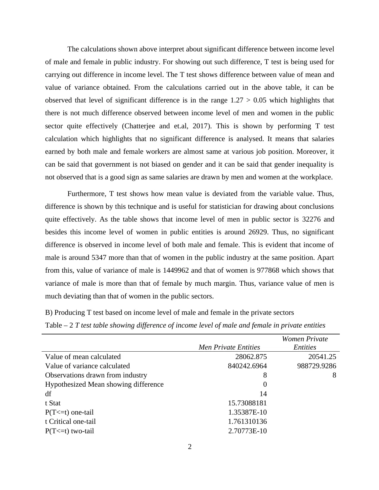
The calculations shown above interpret about significant difference between income level
of male and female in public industry. For showing out such difference, T test is being used for
carrying out difference in income level. The T test shows difference between value of mean and
value of variance obtained. From the calculations carried out in the above table, it can be
observed that level of significant difference is in the range 1.27 > 0.05 which highlights that
there is not much difference observed between income level of men and women in the public
sector quite effectively (Chatterjee and et.al, 2017). This is shown by performing T test
calculation which highlights that no significant difference is analysed. It means that salaries
earned by both male and female workers are almost same at various job position. Moreover, it
can be said that government is not biased on gender and it can be said that gender inequality is
not observed that is a good sign as same salaries are drawn by men and women at the workplace.
Furthermore, T test shows how mean value is deviated from the variable value. Thus,
difference is shown by this technique and is useful for statistician for drawing about conclusions
quite effectively. As the table shows that income level of men in public sector is 32276 and
besides this income level of women in public entities is around 26929. Thus, no significant
difference is observed in income level of both male and female. This is evident that income of
male is around 5347 more than that of women in the public industry at the same position. Apart
from this, value of variance of male is 1449962 and that of women is 977868 which shows that
variance of male is more than that of female by much margin. Thus, variance value of men is
much deviating than that of women in the public sectors.
B) Producing T test based on income level of male and female in the private sectors
Table – 2 T test table showing difference of income level of male and female in private entities
Men Private Entities
Women Private
Entities
Value of mean calculated 28062.875 20541.25
Value of variance calculated 840242.6964 988729.9286
Observations drawn from industry 8 8
Hypothesized Mean showing difference 0
df 14
t Stat 15.73088181
P(T<=t) one-tail 1.35387E-10
t Critical one-tail 1.761310136
P(T<=t) two-tail 2.70773E-10
2

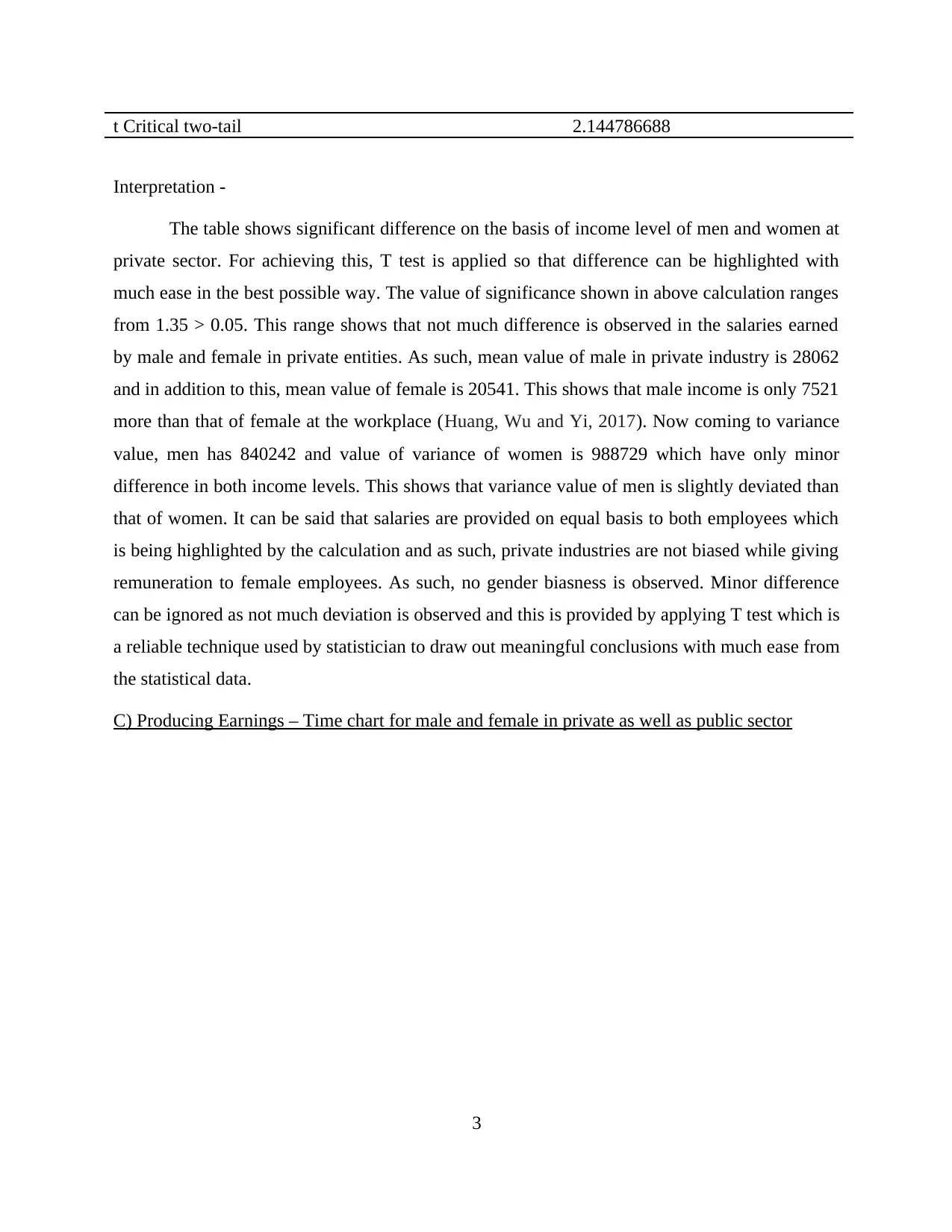
t Critical two-tail 2.144786688
Interpretation -
The table shows significant difference on the basis of income level of men and women at
private sector. For achieving this, T test is applied so that difference can be highlighted with
much ease in the best possible way. The value of significance shown in above calculation ranges
from 1.35 > 0.05. This range shows that not much difference is observed in the salaries earned
by male and female in private entities. As such, mean value of male in private industry is 28062
and in addition to this, mean value of female is 20541. This shows that male income is only 7521
more than that of female at the workplace (Huang, Wu and Yi, 2017). Now coming to variance
value, men has 840242 and value of variance of women is 988729 which have only minor
difference in both income levels. This shows that variance value of men is slightly deviated than
that of women. It can be said that salaries are provided on equal basis to both employees which
is being highlighted by the calculation and as such, private industries are not biased while giving
remuneration to female employees. As such, no gender biasness is observed. Minor difference
can be ignored as not much deviation is observed and this is provided by applying T test which is
a reliable technique used by statistician to draw out meaningful conclusions with much ease from
the statistical data.
C) Producing Earnings – Time chart for male and female in private as well as public sector
3

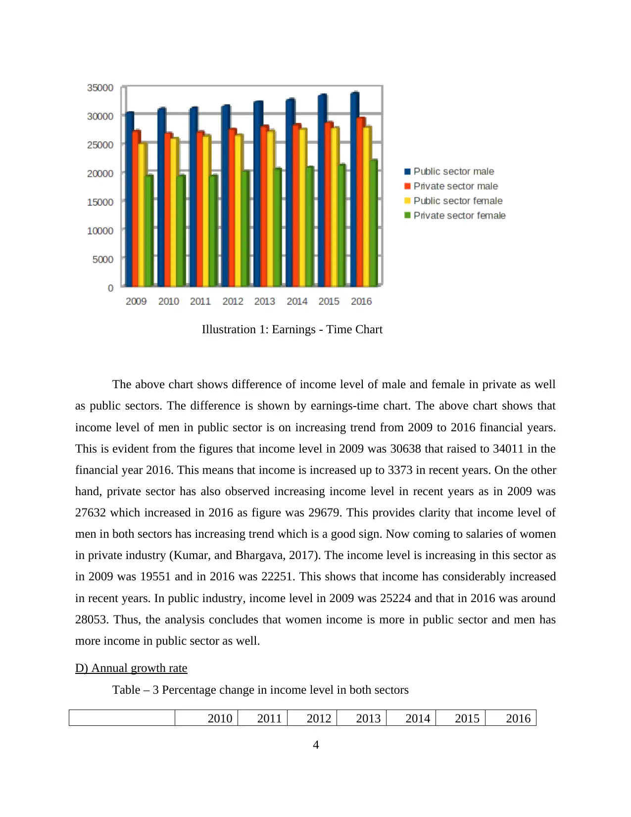
Illustration 1: Earnings - Time Chart
The above chart shows difference of income level of male and female in private as well
as public sectors. The difference is shown by earnings-time chart. The above chart shows that
income level of men in public sector is on increasing trend from 2009 to 2016 financial years.
This is evident from the figures that income level in 2009 was 30638 that raised to 34011 in the
financial year 2016. This means that income is increased up to 3373 in recent years. On the other
hand, private sector has also observed increasing income level in recent years as in 2009 was
27632 which increased in 2016 as figure was 29679. This provides clarity that income level of
men in both sectors has increasing trend which is a good sign. Now coming to salaries of women
in private industry (Kumar, and Bhargava, 2017). The income level is increasing in this sector as
in 2009 was 19551 and in 2016 was 22251. This shows that income has considerably increased
in recent years. In public industry, income level in 2009 was 25224 and that in 2016 was around
28053. Thus, the analysis concludes that women income is more in public sector and men has
more income in public sector as well.
D) Annual growth rate
Table – 3 Percentage change in income level in both sectors
2010 2011 2012 2013 2014 2015 2016
4

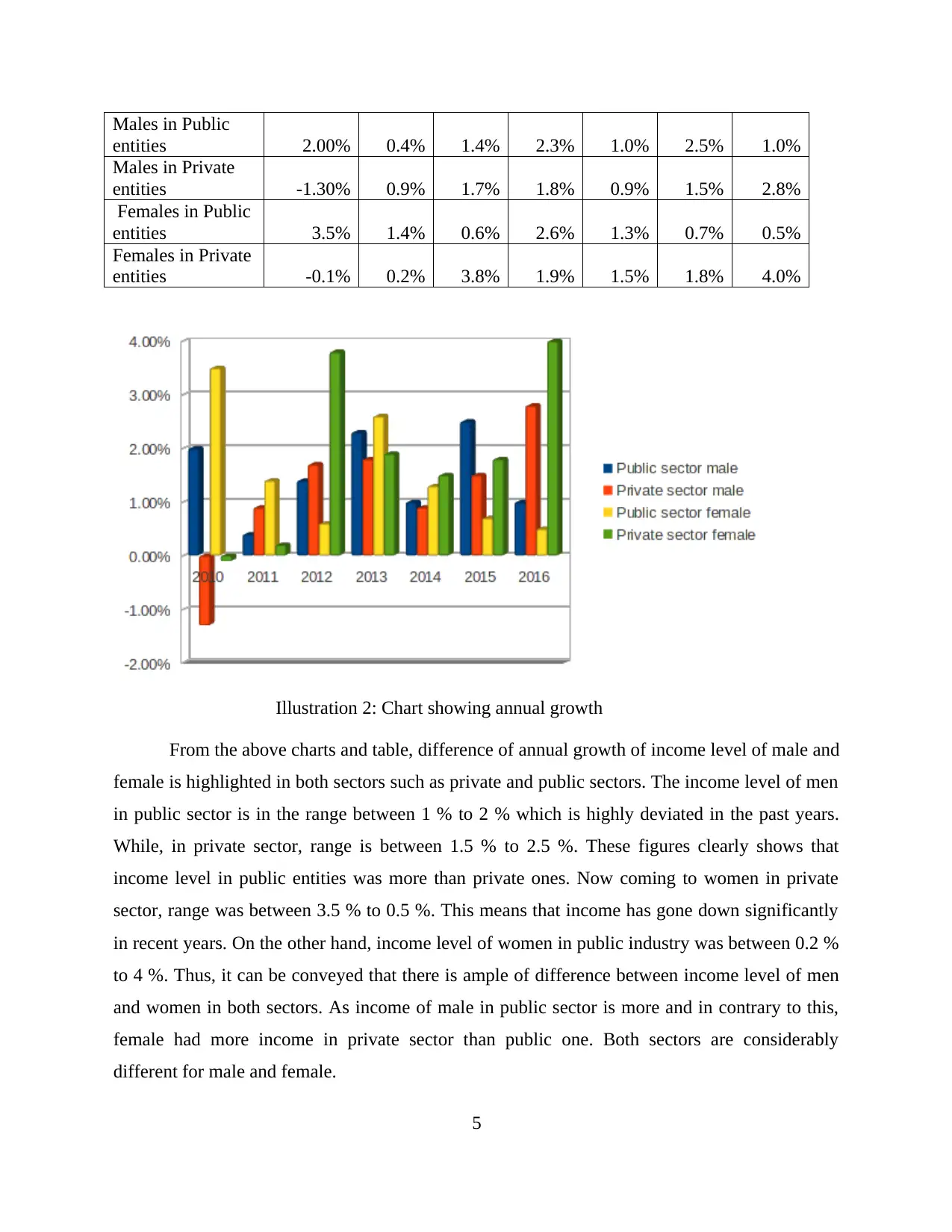
Males in Public
entities 2.00% 0.4% 1.4% 2.3% 1.0% 2.5% 1.0%
Males in Private
entities -1.30% 0.9% 1.7% 1.8% 0.9% 1.5% 2.8%
Females in Public
entities 3.5% 1.4% 0.6% 2.6% 1.3% 0.7% 0.5%
Females in Private
entities -0.1% 0.2% 3.8% 1.9% 1.5% 1.8% 4.0%
Illustration 2: Chart showing annual growth
From the above charts and table, difference of annual growth of income level of male and
female is highlighted in both sectors such as private and public sectors. The income level of men
in public sector is in the range between 1 % to 2 % which is highly deviated in the past years.
While, in private sector, range is between 1.5 % to 2.5 %. These figures clearly shows that
income level in public entities was more than private ones. Now coming to women in private
sector, range was between 3.5 % to 0.5 %. This means that income has gone down significantly
in recent years. On the other hand, income level of women in public industry was between 0.2 %
to 4 %. Thus, it can be conveyed that there is ample of difference between income level of men
and women in both sectors. As income of male in public sector is more and in contrary to this,
female had more income in private sector than public one. Both sectors are considerably
different for male and female.
5

TASK 2
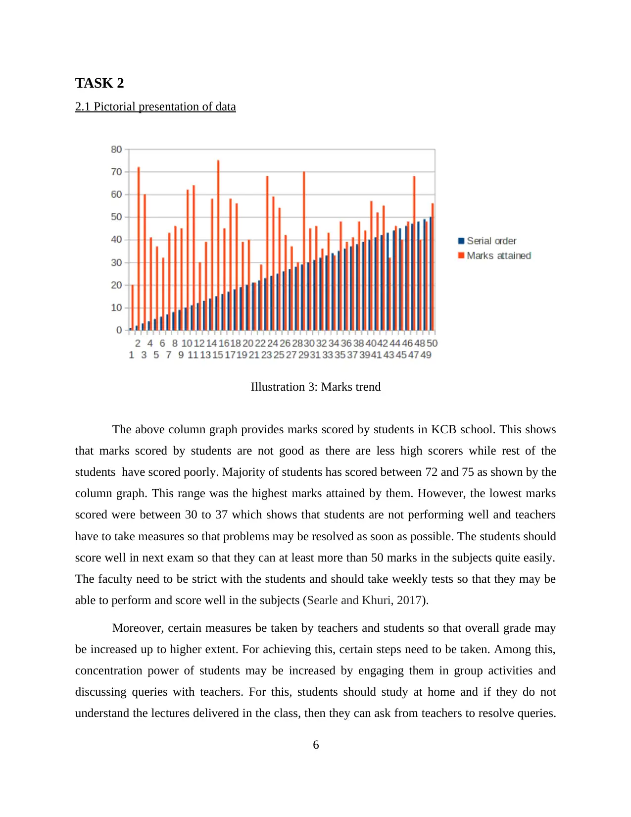
2.1 Pictorial presentation of data
The above column graph provides marks scored by students in KCB school. This shows
that marks scored by students are not good as there are less high scorers while rest of the
students have scored poorly. Majority of students has scored between 72 and 75 as shown by the
column graph. This range was the highest marks attained by them. However, the lowest marks
scored were between 30 to 37 which shows that students are not performing well and teachers
have to take measures so that problems may be resolved as soon as possible. The students should
score well in next exam so that they can at least more than 50 marks in the subjects quite easily.
The faculty need to be strict with the students and should take weekly tests so that they may be
able to perform and score well in the subjects (Searle and Khuri, 2017).
Moreover, certain measures be taken by teachers and students so that overall grade may
be increased up to higher extent. For achieving this, certain steps need to be taken. Among this,
concentration power of students may be increased by engaging them in group activities and
discussing queries with teachers. For this, students should study at home and if they do not
understand the lectures delivered in the class, then they can ask from teachers to resolve queries.
6
Illustration 3: Marks trend

This way grades may be increased effectively. Proper time management may be made by
students so that they may study each subject within stipulated time and this way, syllabus can be
completed within time and students can do revision of the same. Moreover, notes should be
written down by them and this helps to grab things quickly and effectively and students may
scored well in the future. Furthermore, it is not only duty of faculty to make understand value of
studies but parents are equally under duty to guide children so that they may perform well and
achieve good grades.
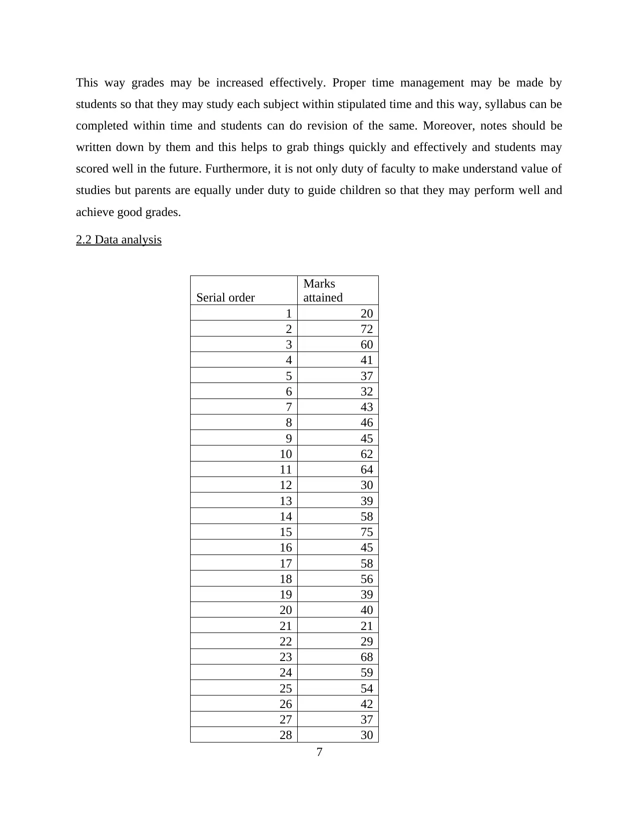
2.2 Data analysis
Serial order
Marks
attained
1 20
2 72
3 60
4 41
5 37
6 32
7 43
8 46
9 45
10 62
11 64
12 30
13 39
14 58
15 75
16 45
17 58
18 56
19 39
20 40
21 21
22 29
23 68
24 59
25 54
26 42
27 37
28 30
7

29 70
30 45
31 46
32 36
33 43
34 33
35 48
36 39
37 41
38 48
39 44
40 57
41 52
42 55
43 32
44 46
45 40
46 48
47 68
48 40
49 48
50 56
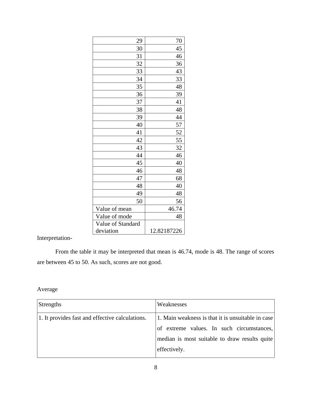
Value of mean 46.74
Value of mode 48
Value of Standard
deviation 12.82187226
Interpretation-
From the table it may be interpreted that mean is 46.74, mode is 48. The range of scores
are between 45 to 50. As such, scores are not good.
Average
Strengths Weaknesses
1. It provides fast and effective calculations. 1. Main weakness is that it is unsuitable in case
of extreme values. In such circumstances,
median is most suitable to draw results quite
effectively.
8

Mode
Strengths Weaknesses
1. It provides data which has occurred most
frequently in the whole data set. This eases to
analyse data in effective way especially, when
data is large enough.
2. It is relevant for qualitative data analysis and
not useful for quantitative data.
1. It does not provide specific range that from
which part value comes most frequently.
2. It is unsuitable for further analysis of data as
it is only once used and not suitable for further
calculations.
B) Discussing measures of dispersion
The measure of central tendency is useful tool but does not provide variable information
of the data. To overcome this shortcoming, measures of dispersion is a useful for statistician to
draw results quite effectively (Measures of Dispersion). Measures of dispersion is the difference
between the smallest score in a data and that of the largest data. It provides better relationship
and combination of data by providing difference between largest and smallest data with much
ease. It has basically two types of it such as absolute and relative measures of dispersion. From
the calculation, it may be analysed that standard deviation calculated is 12 which is deviated
from mean value but moderately only. This makes harder to predict scores of the students. As a
result, it is evident from the fact that measures of dispersion is quite helpful technique to draw
concrete conclusions with much ease.
2.3 Producing report and interpretation of measures of central tendencies
To
The Director of KCB Business School
Subject: Performance of students in the subjects
Mean and mode interpretation
It can be interpreted that mean value obtained is 46. On the other hand, value of mode is 48.
9

This clearly shows that on average, 46 marks have been obtained by students and mode implies
that 48 marks have been scored by most of the students.
Standard deviation
The standard deviation being obtained is 12.82 which can be interpreted that it is moderately
deviated from mean value of 46. This makes prediction of marks to be obtained in future
difficult as standard deviation is moderate and as such, to predict marks is much difficult.
Ways to effectively compare between various subjects
For comparison of subjects, T test can be applied as it provides effective results to easily
compare variables with much ease. Apart from this, ANOVA technique is also useful tool to
compare variables and draw concrete results. This is technique is used to assess difference
between group means. As such, it is good for comparison purpose.
Different ways to assess association
For this, correlation method is quite useful as it provides relationship between two variables and
this is helpful for measuring association with much ease. Another method which can be used is
Chi square test. It is useful tool to measure association and also known as test of independence.
SECTION B
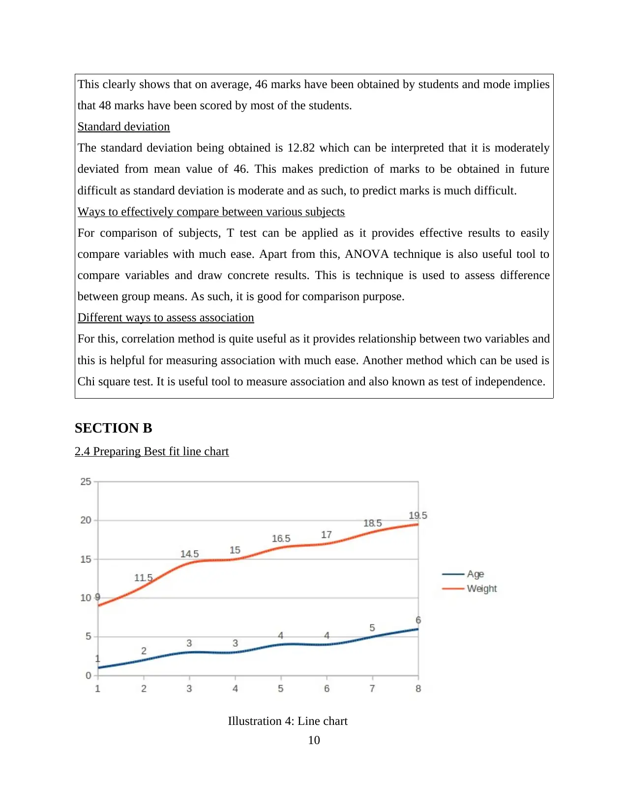
2.4 Preparing Best fit line chart
Illustration 4: Line chart
10