Statistics for Management Report: Data Analysis and Interpretation
VerifiedAdded on 2020/10/05
|11
|3032
|229
Report
AI Summary
This report presents a comprehensive statistical analysis for management, covering various aspects of business operations. It begins with an introduction to business statistics and its importance in decision-making. Activity 1 analyzes changes in gross annual earnings and gender pay gaps in both public and private sectors from 2010 to 2016, providing interpretations of the data. Activity 2 delves into statistical analysis, including the creation of Ogive plots to estimate the median and quartiles of hourly earnings, followed by calculations of mean and standard deviation. Furthermore, the report evaluates hourly pay rates across different regions. Activity 3 focuses on cost-efficient delivery scenarios, evaluating optimal order quantities and total variable costs. The report concludes with a line chart visualization from Activity 1 and provides a summary of the findings, offering valuable insights into data interpretation and business trends.
STATISTICS FOR
MANAGEMENT
MANAGEMENT
Paraphrase This Document
Need a fresh take? Get an instant paraphrase of this document with our AI Paraphraser
Table of Contents
INTRODUCTION...........................................................................................................................1
ACTIVITY 1....................................................................................................................................1
i. Analysing changes in gross annual earnings for public and private sector since 2010.......1
ii. Analysing the gender pay gap for public and private sector..............................................2
ACTIVITY 2....................................................................................................................................3
(a) Ogive Plot to estimate Median for hourly earnings and quartiles.....................................3
i. Median and Inter-Quartile Ranges......................................................................................5
ii. Ascertainment of Mean and Standard Deviation...............................................................5
(b) Evaluation of hourly pay rates..........................................................................................6
ACTIVITY 3....................................................................................................................................7
(a) Current Number of Annual Deliveries..............................................................................7
(b) Number of Bags Delivered...............................................................................................7
(c) Optimal Order Quantity....................................................................................................7
(d) Total Variable Cost...........................................................................................................7
ACTIVITY 4....................................................................................................................................8
Line Chart from Activity 1 for public and private sector.......................................................8
CONCLUSION................................................................................................................................8
REFERENCE...................................................................................................................................9
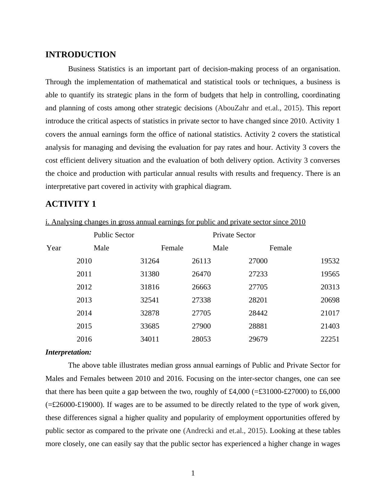
INTRODUCTION
Business Statistics is an important part of decision-making process of an organisation.
Through the implementation of mathematical and statistical tools or techniques, a business is
able to quantify its strategic plans in the form of budgets that help in controlling, coordinating
and planning of costs among other strategic decisions (AbouZahr and et.al., 2015). This report
introduce the critical aspects of statistics in private sector to have changed since 2010. Activity 1
covers the annual earnings form the office of national statistics. Activity 2 covers the statistical
analysis for managing and devising the evaluation for pay rates and hour. Activity 3 covers the
cost efficient delivery situation and the evaluation of both delivery option. Activity 3 converses
the choice and production with particular annual results with results and frequency. There is an
interpretative part covered in activity with graphical diagram.
ACTIVITY 1
i. Analysing changes in gross annual earnings for public and private sector since 2010
Public Sector Private Sector
Year Male Female Male Female
2010 31264 26113 27000 19532
2011 31380 26470 27233 19565
2012 31816 26663 27705 20313
2013 32541 27338 28201 20698
2014 32878 27705 28442 21017
2015 33685 27900 28881 21403
2016 34011 28053 29679 22251
Interpretation:
The above table illustrates median gross annual earnings of Public and Private Sector for
Males and Females between 2010 and 2016. Focusing on the inter-sector changes, one can see
that there has been quite a gap between the two, roughly of £4,000 (=£31000-£27000) to £6,000
(=£26000-£19000). If wages are to be assumed to be directly related to the type of work given,
these differences signal a higher quality and popularity of employment opportunities offered by
public sector as compared to the private one (Andrecki and et.al., 2015). Looking at these tables
more closely, one can easily say that the public sector has experienced a higher change in wages
1
⊘ This is a preview!⊘
Do you want full access?
Subscribe today to unlock all pages.
Trusted by 1+ million students worldwide
as compared to private sector. For instance, the annual earnings for Females in Public Sector
amounted to £28,053 whereas for Private Sector it was £22,251. This clearly shows a difference
of roughly £6,000 between the two. Also if the wages of each gender in respective sectors have
to be taken into consideration, there has been a growth of 8.79% for Men in Public Sector and
9.92% in Private. Similarly, there has been a 7.43% growth in Females' Earnings for the same
period in Public Sector and 13.92% growth in Private Sector. This shows that the sectors have
been experiencing a positive growth trend with more growth opportunities in Private Sector even
though the wages earned by both genders is higher for Public Sector.
ii. Analysing the gender pay gap for public and private sector
Public Sector:
Public Sector Gap Gap (%)
Year Males Females
2010 31264 26113 5151
2011 31380 26470 4910 -4.68%
2012 31816 26663 5153 4.95%
2013 32541 27338 5203 0.97%
2014 32878 27705 5173 -0.58%
2015 33685 27900 5785 11.83%
2016 34011 28053 5958 2.99%
Interpretation:
The aforementioned table gives a comprehensive look at the gender pay gaps prevalent in
the Public Sector. The gap column indicates the changes in gross annual earnings for males and
females for each year. Looking closely at this column one can see a fluctuating trend for the two
genders between 2010 and 2016. The last column of this table quantifies the gap in terms of
percentage to show the change in gaps for males and females' median gross annual earnings for
the chosen time period. The highest change is experienced in 2015 where the gap increased by
almost £600 from previous year. This can be mainly attributed to the rise in earnings of men
which is £807 (=£33685-£32878) which is higher than the change in women's earnings
amounting to mere £205 (=£27900-£27705). Taking into consideration the entire time frame
there has been a rise of gap by roughly £800 which is quite substantial for the sector (Brewster
and Hegewisch, 2017).
2
Paraphrase This Document
Need a fresh take? Get an instant paraphrase of this document with our AI Paraphraser
Private Sector:
Private Sector Gap Gap (%)
Year Males Women
2010 27000 19532 7468
2011 27233 19565 7668 2.68%
2012 27705 20313 7392 -3.60%
2013 28201 20698 7503 1.50%
2014 28442 21017 7425 -1.04%
2015 28881 21403 7478 0.71%
2016 29679 22251 7428 -0.67%
Interpretation:
Private Sector is mostly governed with Public Limited Companies, Franchises, Sole
Proprietorships, Partnerships among other organisations. Hence, there is a higher competition
prevalent in the business environment (Chen, Cheng and Wang, 2015). This leads to a higher
demand for extremely knowledgable and specialised workforce. It can be seen that the gap has
been almost constant for this sector over the years. In fact, it has reduced to £7428 from £7468
since 2010. Even though the reduction is not that substantial it indicates a trend of reducing pay
gaps for males and females and an increase in equity for both among the top management of
players operative in such industry.
ACTIVITY 2
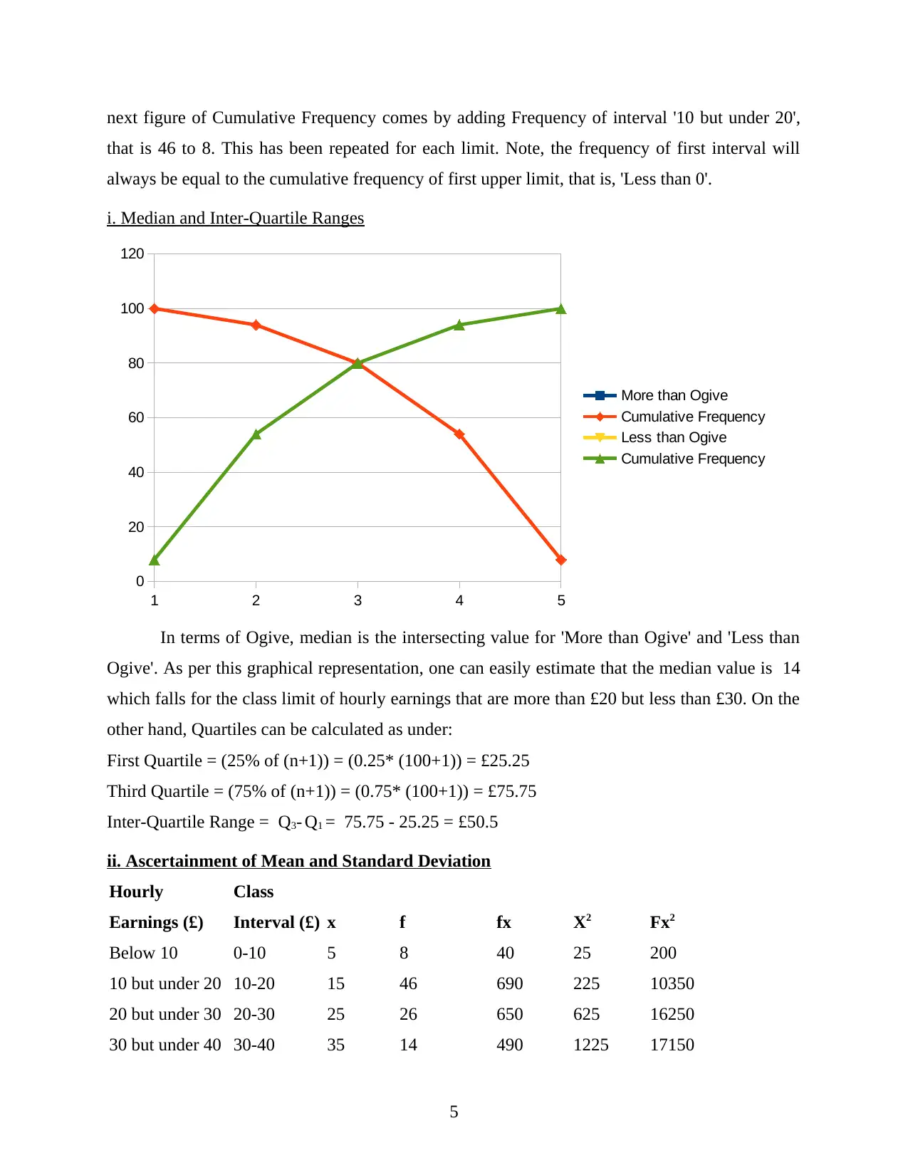
(a) Ogive Plot to estimate Median for hourly earnings and quartiles
Ogive is a graphical representation of Cumulative Frequencies in order to ascertain
Median. It helps in affirming that the researcher has included all the important variables while
deriving the results from collected sample or not. In order to estimate Median, a 'More than
Ogive' and ' Less than Ogive' are created and their intersection point is taken as the middle value
(Ismyrlis, Moschidis and Tsiotras, 2015). For this purpose, the following table has been
converted into a More than and Less than Ogive tabulations:
Hourly Earnings (£) % of Employees
Cumulative
Frequency
Below 10 8 8
3
Private Sector Gap Gap (%)
Year Males Women
2010 27000 19532 7468
2011 27233 19565 7668 2.68%
2012 27705 20313 7392 -3.60%
2013 28201 20698 7503 1.50%
2014 28442 21017 7425 -1.04%
2015 28881 21403 7478 0.71%
2016 29679 22251 7428 -0.67%
Interpretation:
Private Sector is mostly governed with Public Limited Companies, Franchises, Sole
Proprietorships, Partnerships among other organisations. Hence, there is a higher competition
prevalent in the business environment (Chen, Cheng and Wang, 2015). This leads to a higher
demand for extremely knowledgable and specialised workforce. It can be seen that the gap has
been almost constant for this sector over the years. In fact, it has reduced to £7428 from £7468
since 2010. Even though the reduction is not that substantial it indicates a trend of reducing pay
gaps for males and females and an increase in equity for both among the top management of
players operative in such industry.
ACTIVITY 2
(a) Ogive Plot to estimate Median for hourly earnings and quartiles
Ogive is a graphical representation of Cumulative Frequencies in order to ascertain
Median. It helps in affirming that the researcher has included all the important variables while
deriving the results from collected sample or not. In order to estimate Median, a 'More than
Ogive' and ' Less than Ogive' are created and their intersection point is taken as the middle value
(Ismyrlis, Moschidis and Tsiotras, 2015). For this purpose, the following table has been
converted into a More than and Less than Ogive tabulations:
Hourly Earnings (£) % of Employees
Cumulative
Frequency
Below 10 8 8
3
10 but under 20 46 54
20 but under 30 26 80
30 but under 40 14 94
40 but under 50 6 100
More than Ogive:
Hourly Earning (£) % of Employees More than Ogive Cumulative Frequency
Below 10 8 More than 0 100
10 but under 20 46 More than 10 94
20 but under 30 26 More than 20 80
30 but under 40 14 More than 30 54
40 but under 50 6 More than 40 8
Total 100
A 'More than Ogive' is one which includes Cumulative Frequencies calculated from
below including the lower class limits and their related additive frequency values. For 'More than
0' the cumulative frequency is at 100 (Jennings, Nagel and Mansfield 2016). For 'More than 10',
the cumulative frequency comes by subtracting Frequency of interval '10 but under 20', that is 8,
from 100. This has been repeated for each limit. Note, the frequency of first interval will always
be equal to the cumulative frequency of last lower limit, that is, 'More than 40'.
Less than Ogive:
Hourly Earning (£) % of Employees Less than Ogive Cumulative Frequency
Below 10 8 Less than 0 8
10 but under 20 46 Less than 10 54
20 but under 30 26 Less than 20 80
30 but under 40 14 Less than 30 94
40 but under 50 6 Less than 40 100
Total 100
A 'Less than Ogive' is one which includes Cumulative Frequencies calculated from above
including the upper class limits and their related additive frequency values. For 'Less than 0' the
cumulative frequency is at 8 (Lo, Ramos and Rogo, 2017). For 'Less than 10', the cumulative
frequency is equal to the cumulative frequency of first upper class limit in 'Less than 40'. The
4
⊘ This is a preview!⊘
Do you want full access?
Subscribe today to unlock all pages.
Trusted by 1+ million students worldwide
next figure of Cumulative Frequency comes by adding Frequency of interval '10 but under 20',
that is 46 to 8. This has been repeated for each limit. Note, the frequency of first interval will
always be equal to the cumulative frequency of first upper limit, that is, 'Less than 0'.
i. Median and Inter-Quartile Ranges
1 2 3 4 5
0
20
40
60
80
100
120
More than Ogive
Cumulative Frequency
Less than Ogive
Cumulative Frequency
In terms of Ogive, median is the intersecting value for 'More than Ogive' and 'Less than
Ogive'. As per this graphical representation, one can easily estimate that the median value is 14
which falls for the class limit of hourly earnings that are more than £20 but less than £30. On the
other hand, Quartiles can be calculated as under:
First Quartile = (25% of (n+1)) = (0.25* (100+1)) = £25.25
Third Quartile = (75% of (n+1)) = (0.75* (100+1)) = £75.75
Inter-Quartile Range = Q3- Q1 = 75.75 - 25.25 = £50.5
ii. Ascertainment of Mean and Standard Deviation
Hourly
Earnings (£)
Class
Interval (£) x f fx X2 Fx2
Below 10 0-10 5 8 40 25 200
10 but under 20 10-20 15 46 690 225 10350
20 but under 30 20-30 25 26 650 625 16250
30 but under 40 30-40 35 14 490 1225 17150
5
Paraphrase This Document
Need a fresh take? Get an instant paraphrase of this document with our AI Paraphraser
40 but under 50 40-50 45 6 270 2025 12150
100 2140 56100
Interpretation:
Mean is the average value for a given sample data. The above table includes an exclusive
class interval series, hence, the 'x' value needs to be found out. This has been calculated by
adding the limits and dividing them by 2 (McCaffery, 2018). Therefore, x for class interval £0 to
£10 is 5, £10 to £20 is 15 and so on. Frequency or 'f' denotes the percentage of employees. The
Mean value for the given data set is computed as follows:
Mean = ∑fx / ∑f where,
∑fx = Summation of (Frequency * Central Interval Point)
∑f = Total percentage of Employees
Mean = 2140/100 = 21.40 or 22 employees.
Standard Deviation is the measure of dispersion indicating how far the data values spread
from the mean. Hence, it is calculated as under:
Standard deviation = √ (∑fx2 / ∑f) - (∑fx / ∑f)2 where,
∑fx2 = Summation of Squared (frequency * central interval point)
∑f = Total percentage of Employees
(∑fx / ∑f)2 = Squared Mean
Standard deviation = √ (∑Fx2 / ∑F) - (∑Fx / ∑F)2 = √[(56100/100) – (21.4)2 ]= √[561 – 457.96]
= √103.04 = 10.15
(b) Evaluation of hourly pay rates
Survey Regions North-East South-West
Median 14.5 14
Inter-Quartile Range 8 50.5
Mean 16.7 21.4
Standard Deviation 7.4 10.15
Interpretation:
As per the survey results derived from North-East and South-West Regions, the
aforementioned measures of central tendency and dispersion. The median value for both regions
is almost close, hence, one can say that the data collected for both the regions have similar
characteristics and the values for both fall in almost similar areas (McNeil, Frey and Embrechts,
6
2015). As the sample data values is more in South-West, it has a higher inter-quartile range as
compared to North-East. The average earnings for North-East is lower than the South-West
indicating that there is much more scope for employees in terms of earning opportunities as
compared to north-east region. However, the standard Deviation from Mean is more for South-
West Region signalling a higher fluctuation in prices from the average earnings for that region.
ACTIVITY 3
(a) Current Number of Annual Deliveries
EOQ is an inventory model that helps to define excess stock and when an organisation
should place order to purchase products during engaging in production process (Schwalbe,
2015). In given context supplier delivers rice very twelve days at the cost of £20. and market
closed on five days each year. Therefore, it make deliveries in a current year:-
Number of day sin a year 365
Closed day 5
Deliver rice during gaps 12
Number of current year delivery 365-5/12= 30 deliveries
(b) Number of Bags Delivered
number of rice bags that can be delivered= [(Annual demand / EOQ)]
= 45000/ 134.164
= 33.54
Therefore, a supplier can deliver 33.54 bags of rice in a current year.
(c) Optimal Order Quantity
Economic order quantity: = 2* √U*O/C
= 2* √45000*2/20
= 134.164
(d) Total Variable Cost
Annual Ordering Cost = Number of Orders* Cost per Order
=30*£20 = £600
7
⊘ This is a preview!⊘
Do you want full access?
Subscribe today to unlock all pages.
Trusted by 1+ million students worldwide
Annual Carrying Cost = Average Inventory* Annual Carrying Cost per unit
= (45000/2)*(0.25*£2) = 22500*£0.5 = £11250
From above calculations one can say that the total variable cost model is £11,850 which
is the cost of implementing the current policy in terms of Economic Order Quantity that the
seller wishes to maintain (Shanks, 2016).
ACTIVITY 4
Line Chart from Activity 1 for public and private sector
02/07/1905 04/07/1905 06/07/1905 08/07/1905
0
5000
10000
15000
20000
25000
30000
35000
40000
Public Sector Male
Female
Private Sector Male
Female
CONCLUSION
The above mentioned report give a summary of methodologies that run by a business
entities of different size and nature in order to operation management. This report also define
cases in which business thoughts can be derived from published sources for substantive
information. It also considered ascertainment of deviation and economic models that provides a
statical information. It revealed that an organisation should adopt inventory management system
that helps to minimize industry's cost by applying Economic order quantity model which states
that when an industry should place a order to purchase raw material. Moreover, this report
covered CPI and RPI that can be understand easily through chart and shows important figure for
managing in a proper manner.
8
Paraphrase This Document
Need a fresh take? Get an instant paraphrase of this document with our AI Paraphraser

9
1 out of 11
Related Documents


Your All-in-One AI-Powered Toolkit for Academic Success.
+13062052269
info@desklib.com
Available 24*7 on WhatsApp / Email
![[object Object]](/_next/static/media/star-bottom.7253800d.svg)
Unlock your academic potential
Copyright © 2020–2026 A2Z Services. All Rights Reserved. Developed and managed by ZUCOL.