Statistics for Management: Data Analysis and Growth Rate Report
VerifiedAdded on 2020/10/05
|23
|5374
|166
Report
AI Summary
This report on Statistics for Management delves into various statistical techniques used in business decision-making. It begins with an introduction to statistics and its application in organizations. The report is divided into four tasks: Task 1 focuses on hypothesis testing, comparing earnings between men and women in both public and private sectors, generating earnings-time charts, and calculating annual growth rates. Task 2 explores cumulative histograms for estimating median and quartiles, and computing central tendency and dispersion. Task 3 addresses inventory management, including computing optimal stock levels, ordering quantities, inventory costs, and service levels. Finally, the report concludes with a summary of findings and references.

STATISTICS FOR
MANAGEMENT
MANAGEMENT
Paraphrase This Document
Need a fresh take? Get an instant paraphrase of this document with our AI Paraphraser
Table of Contents
INTRODUCTION...........................................................................................................................1
TASK 1............................................................................................................................................1
(a) Investigating Hypothesis under Public Sector.......................................................................1
(b) Investigating Hypothesis under Private Sector......................................................................3
(c) Using excel to generate Earnings-Time Chart for each group..............................................4
(d) Calculation of Annual Growth Rate......................................................................................6
.........................................................................................................................................................7
TASK 2............................................................................................................................................9
(i) Employing Cumulative Histogram in estimation of Median and Quartiles for Leisure
Centre..........................................................................................................................................9
Computation of Additive Frequency...........................................................................................9
Ogive.........................................................................................................................................10
(ii) Computation of Central Tendency and Dispersion:............................................................13
(a) Comparison between the statistical measurements of two leisure centre............................14
TASK 3..........................................................................................................................................15
(a) Computing optimal level of stock .......................................................................................15
(b) Number of Orders to be placed for tee-shirts......................................................................16
(c) Computing Inventory Policy Cost.......................................................................................16
(d) Current Service Level to Customers....................................................................................17
(e) Ascertaining re-ordering levels to fulfil desired service levels...........................................17
TASK 4..........................................................................................................................................17
CONCLUSION..............................................................................................................................20
REFERENCES..............................................................................................................................21
INTRODUCTION
Statistics relates to the tools and techniques used in the process of decision-making in an
organisation. It takes into account important information derived in the form of qualitative and
quantitative data to draw conclusions and take strategic actions by the business. Utilization of
statistics in a business scenario helps in increasing productivity, reducing costs and measuring
uncertainty in a scientific manner (Baglin and Da Costa, 2012).
This report aims at depicting detailed account in regards to the measures of central
tendency, dispersion and variability. Moreover, the report is divided into four tasks which relate
to hypothesis testing, ogive, inventory management model and production of charts through data
collected.
TASK 1
The term 'hypothesis' refers to a statement or explanation proposed in relation to the
happening or non-happening of a particular event. A hypothesis is usually formed on the basis of
past experiences, observations and data collected to infer judgements regarding the given
statement. In the context of Business Statistics, this methodology is adopted in order to
experiment with various assumptions and plans undertaken by the organisation to ascertain how
successful they would be in implementation of such scenarios in the real world (Borio, 2013).
When forming a hypothesis, a researcher usually takes two scenarios for the proposed
explanation. One that is true (H0) and one that is not (H1). Hereafter, the researcher employs
appropriate statistical techniques in order to spot patterns and connect information to ascertain
whether the formed hypothesis is true or not. In case, the hypothesis proves to be true, it is said
that H0 is accepted and H1 is rejected. This process of experimentation is known as 'Investigation
of Hypothesis' (BOUKACEM‐ZEGHMOURI and Schöpfel, 2012).
For the given case scenario, the data has been extracted for public as well as private
sector and has been construed on the basis of sex. The following hypothesis have been
formulated in each scenario to ascertain the truth in such assertions:
(a) Investigating Hypothesis under Public Sector
Under this scenario, the following hypothesis has been formulated:
H0: Earnings of men is not substantially higher to that of women in Public Sector.
H1: Earnings of men is substantially higher to that of women in Public Sector.
1
⊘ This is a preview!⊘
Do you want full access?
Subscribe today to unlock all pages.
Trusted by 1+ million students worldwide
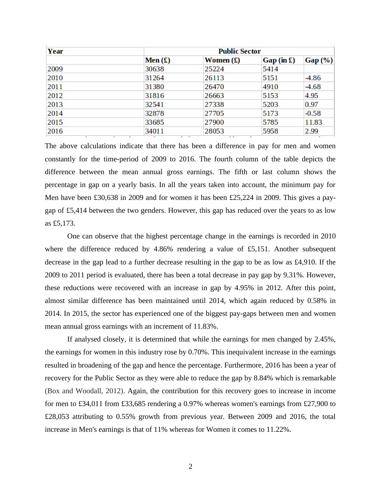
The above calculations indicate that there has been a difference in pay for men and women
constantly for the time-period of 2009 to 2016. The fourth column of the table depicts the
difference between the mean annual gross earnings. The fifth or last column shows the
percentage in gap on a yearly basis. In all the years taken into account, the minimum pay for
Men have been £30,638 in 2009 and for women it has been £25,224 in 2009. This gives a pay-
gap of £5,414 between the two genders. However, this gap has reduced over the years to as low
as £5,173.
One can observe that the highest percentage change in the earnings is recorded in 2010
where the difference reduced by 4.86% rendering a value of £5,151. Another subsequent
decrease in the gap lead to a further decrease resulting in the gap to be as low as £4,910. If the
2009 to 2011 period is evaluated, there has been a total decrease in pay gap by 9.31%. However,
these reductions were recovered with an increase in gap by 4.95% in 2012. After this point,
almost similar difference has been maintained until 2014, which again reduced by 0.58% in
2014. In 2015, the sector has experienced one of the biggest pay-gaps between men and women
mean annual gross earnings with an increment of 11.83%.
If analysed closely, it is determined that while the earnings for men changed by 2.45%,
the earnings for women in this industry rose by 0.70%. This inequivalent increase in the earnings
resulted in broadening of the gap and hence the percentage. Furthermore, 2016 has been a year of
recovery for the Public Sector as they were able to reduce the gap by 8.84% which is remarkable
(Box and Woodall, 2012). Again, the contribution for this recovery goes to increase in income
for men to £34,011 from £33,685 rendering a 0.97% whereas women's earnings from £27,900 to
£28,053 attributing to 0.55% growth from previous year. Between 2009 and 2016, the total
increase in Men's earnings is that of 11% whereas for Women it comes to 11.22%.
2
Paraphrase This Document
Need a fresh take? Get an instant paraphrase of this document with our AI Paraphraser
One the basis of these findings, it can be concluded that the earnings of men are not
substantially higher than that of women employed in the Public Sector. This means that H0 is
accepted and H1 is rejected.
(b) Investigating Hypothesis under Private Sector
Under this scenario, the following hypothesis has been formulated:
H0: Earnings of men is not substantially higher to that of women in Private Sector.
H1: Earnings of men is substantially higher to that of women in Private Sector.
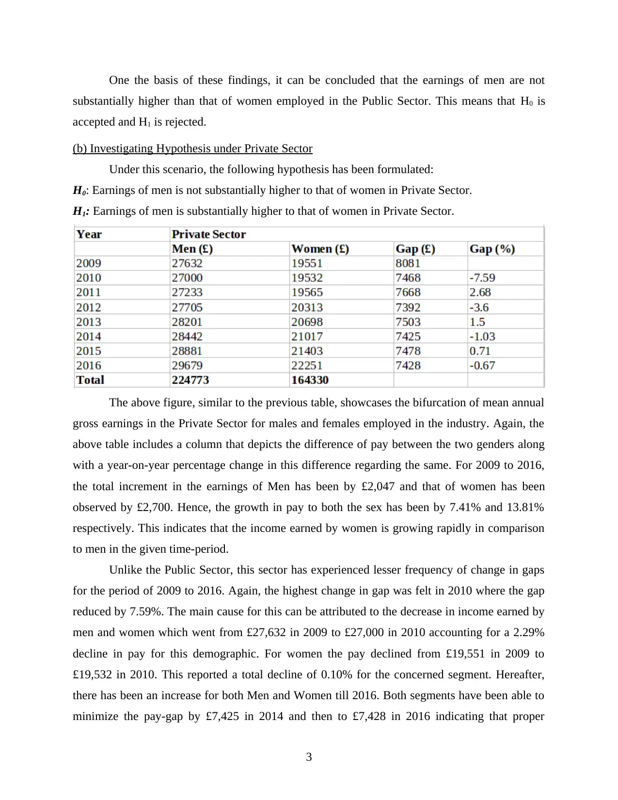
The above figure, similar to the previous table, showcases the bifurcation of mean annual
gross earnings in the Private Sector for males and females employed in the industry. Again, the
above table includes a column that depicts the difference of pay between the two genders along
with a year-on-year percentage change in this difference regarding the same. For 2009 to 2016,
the total increment in the earnings of Men has been by £2,047 and that of women has been
observed by £2,700. Hence, the growth in pay to both the sex has been by 7.41% and 13.81%
respectively. This indicates that the income earned by women is growing rapidly in comparison
to men in the given time-period.
Unlike the Public Sector, this sector has experienced lesser frequency of change in gaps
for the period of 2009 to 2016. Again, the highest change in gap was felt in 2010 where the gap
reduced by 7.59%. The main cause for this can be attributed to the decrease in income earned by
men and women which went from £27,632 in 2009 to £27,000 in 2010 accounting for a 2.29%
decline in pay for this demographic. For women the pay declined from £19,551 in 2009 to
£19,532 in 2010. This reported a total decline of 0.10% for the concerned segment. Hereafter,
there has been an increase for both Men and Women till 2016. Both segments have been able to
minimize the pay-gap by £7,425 in 2014 and then to £7,428 in 2016 indicating that proper
3
substantially higher than that of women employed in the Public Sector. This means that H0 is
accepted and H1 is rejected.
(b) Investigating Hypothesis under Private Sector
Under this scenario, the following hypothesis has been formulated:
H0: Earnings of men is not substantially higher to that of women in Private Sector.
H1: Earnings of men is substantially higher to that of women in Private Sector.
The above figure, similar to the previous table, showcases the bifurcation of mean annual
gross earnings in the Private Sector for males and females employed in the industry. Again, the
above table includes a column that depicts the difference of pay between the two genders along
with a year-on-year percentage change in this difference regarding the same. For 2009 to 2016,
the total increment in the earnings of Men has been by £2,047 and that of women has been
observed by £2,700. Hence, the growth in pay to both the sex has been by 7.41% and 13.81%
respectively. This indicates that the income earned by women is growing rapidly in comparison
to men in the given time-period.
Unlike the Public Sector, this sector has experienced lesser frequency of change in gaps
for the period of 2009 to 2016. Again, the highest change in gap was felt in 2010 where the gap
reduced by 7.59%. The main cause for this can be attributed to the decrease in income earned by
men and women which went from £27,632 in 2009 to £27,000 in 2010 accounting for a 2.29%
decline in pay for this demographic. For women the pay declined from £19,551 in 2009 to
£19,532 in 2010. This reported a total decline of 0.10% for the concerned segment. Hereafter,
there has been an increase for both Men and Women till 2016. Both segments have been able to
minimize the pay-gap by £7,425 in 2014 and then to £7,428 in 2016 indicating that proper
3
measures have been taken by industry players to control the gap and encourage recognition as
well as equality in the work environment for both genders (George, Haas and Pentland, 2014).
On the basis of such observations, the hypothesis holds true for the data extracted
resulting in acceptance of H0 while H1 is rejected.
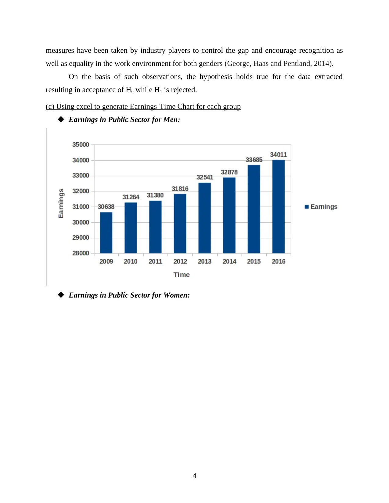
(c) Using excel to generate Earnings-Time Chart for each group
Earnings in Public Sector for Men:
Earnings in Public Sector for Women:
4
well as equality in the work environment for both genders (George, Haas and Pentland, 2014).
On the basis of such observations, the hypothesis holds true for the data extracted
resulting in acceptance of H0 while H1 is rejected.
(c) Using excel to generate Earnings-Time Chart for each group
Earnings in Public Sector for Men:
Earnings in Public Sector for Women:
4
⊘ This is a preview!⊘
Do you want full access?
Subscribe today to unlock all pages.
Trusted by 1+ million students worldwide
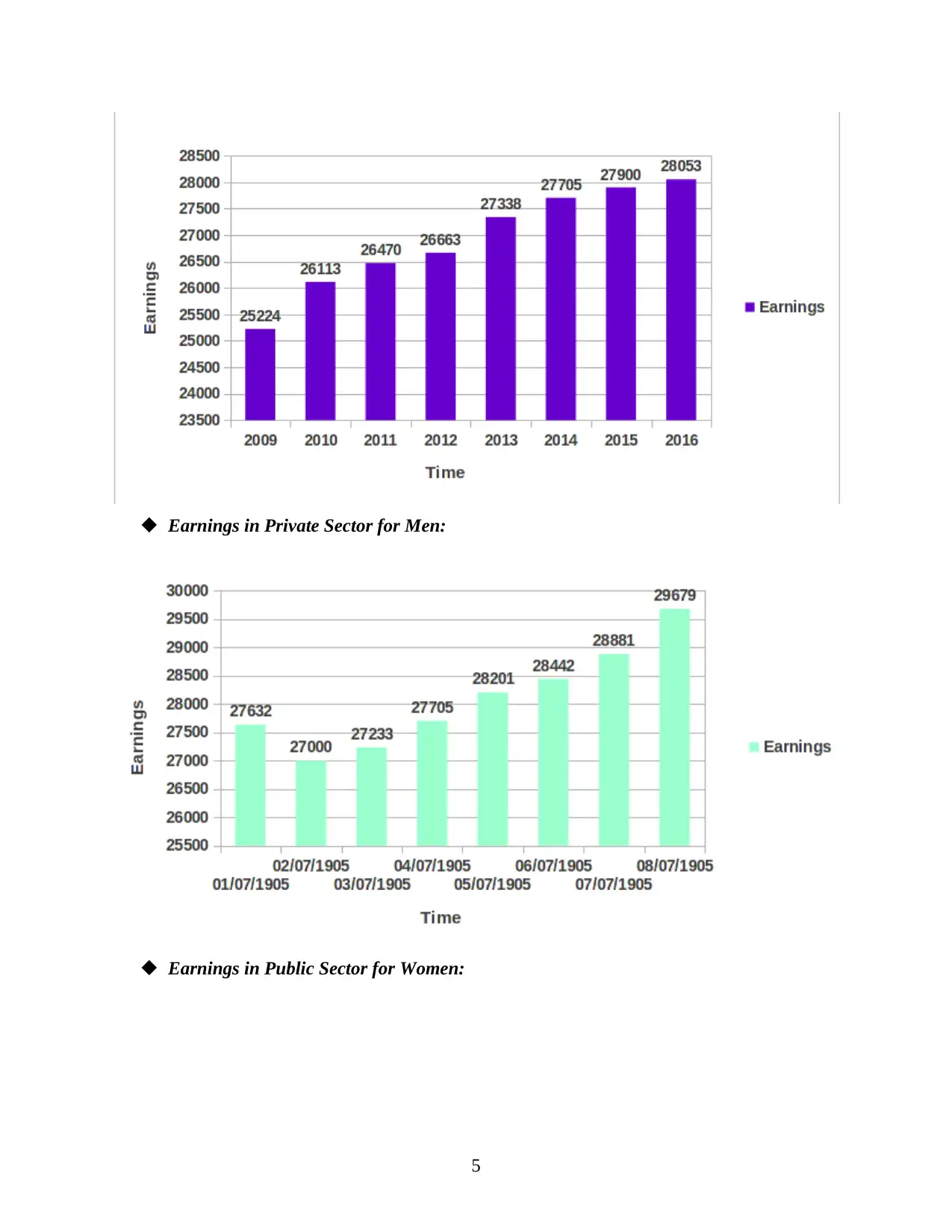
Earnings in Private Sector for Men:
Earnings in Public Sector for Women:
5
Earnings in Public Sector for Women:
5
Paraphrase This Document
Need a fresh take? Get an instant paraphrase of this document with our AI Paraphraser
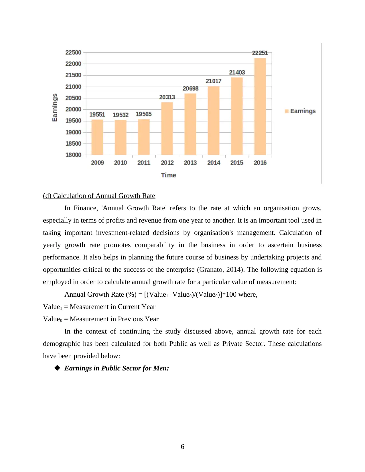
(d) Calculation of Annual Growth Rate
In Finance, 'Annual Growth Rate' refers to the rate at which an organisation grows,
especially in terms of profits and revenue from one year to another. It is an important tool used in
taking important investment-related decisions by organisation's management. Calculation of
yearly growth rate promotes comparability in the business in order to ascertain business
performance. It also helps in planning the future course of business by undertaking projects and
opportunities critical to the success of the enterprise (Granato, 2014). The following equation is
employed in order to calculate annual growth rate for a particular value of measurement:
Annual Growth Rate (%) = [(Value1- Value0)/(Value0)]*100 where,
Value1 = Measurement in Current Year
Value0 = Measurement in Previous Year
In the context of continuing the study discussed above, annual growth rate for each
demographic has been calculated for both Public as well as Private Sector. These calculations
have been provided below:
Earnings in Public Sector for Men:
6
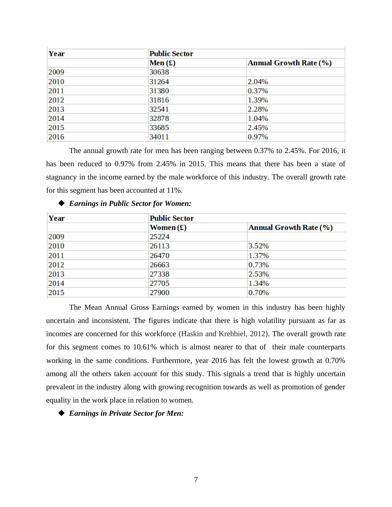
The annual growth rate for men has been ranging between 0.37% to 2.45%. For 2016, it
has been reduced to 0.97% from 2.45% in 2015. This means that there has been a state of
stagnancy in the income earned by the male workforce of this industry. The overall growth rate
for this segment has been accounted at 11%.
Earnings in Public Sector for Women:
The Mean Annual Gross Earnings earned by women in this industry has been highly
uncertain and inconsistent. The figures indicate that there is high volatility pursuant as far as
incomes are concerned for this workforce (Haskin and Krehbiel, 2012). The overall growth rate
for this segment comes to 10.61% which is almost nearer to that of their male counterparts
working in the same conditions. Furthermore, year 2016 has felt the lowest growth at 0.70%
among all the others taken account for this study. This signals a trend that is highly uncertain
prevalent in the industry along with growing recognition towards as well as promotion of gender
equality in the work place in relation to women.
Earnings in Private Sector for Men:
7
⊘ This is a preview!⊘
Do you want full access?
Subscribe today to unlock all pages.
Trusted by 1+ million students worldwide
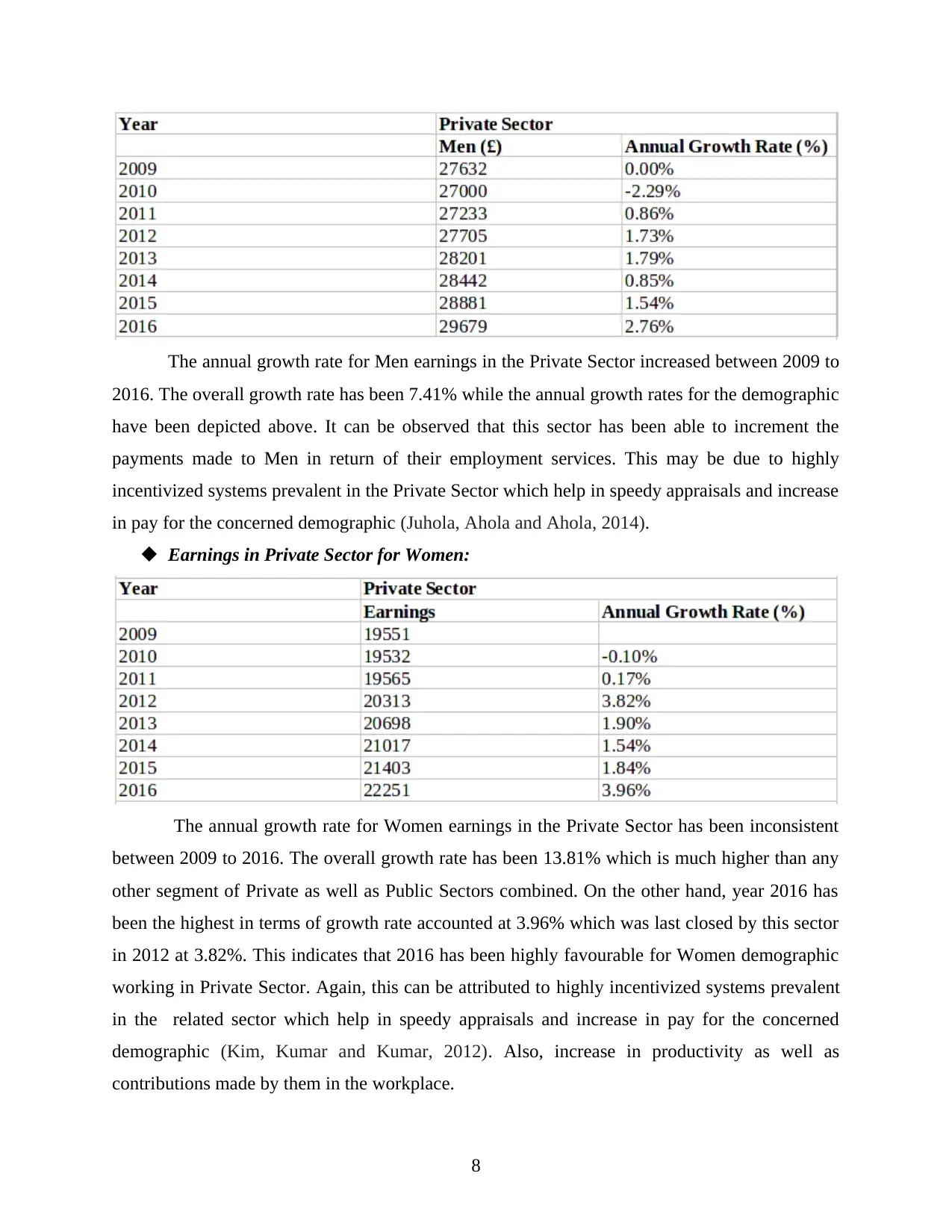
The annual growth rate for Men earnings in the Private Sector increased between 2009 to
2016. The overall growth rate has been 7.41% while the annual growth rates for the demographic
have been depicted above. It can be observed that this sector has been able to increment the
payments made to Men in return of their employment services. This may be due to highly
incentivized systems prevalent in the Private Sector which help in speedy appraisals and increase
in pay for the concerned demographic (Juhola, Ahola and Ahola, 2014).
Earnings in Private Sector for Women:
The annual growth rate for Women earnings in the Private Sector has been inconsistent
between 2009 to 2016. The overall growth rate has been 13.81% which is much higher than any
other segment of Private as well as Public Sectors combined. On the other hand, year 2016 has
been the highest in terms of growth rate accounted at 3.96% which was last closed by this sector
in 2012 at 3.82%. This indicates that 2016 has been highly favourable for Women demographic
working in Private Sector. Again, this can be attributed to highly incentivized systems prevalent
in the related sector which help in speedy appraisals and increase in pay for the concerned
demographic (Kim, Kumar and Kumar, 2012). Also, increase in productivity as well as
contributions made by them in the workplace.
8
Paraphrase This Document
Need a fresh take? Get an instant paraphrase of this document with our AI Paraphraser
TASK 2
(i) Employing Cumulative Histogram in estimation of Median and Quartiles for Leisure Centre
Computation of Additive Frequency
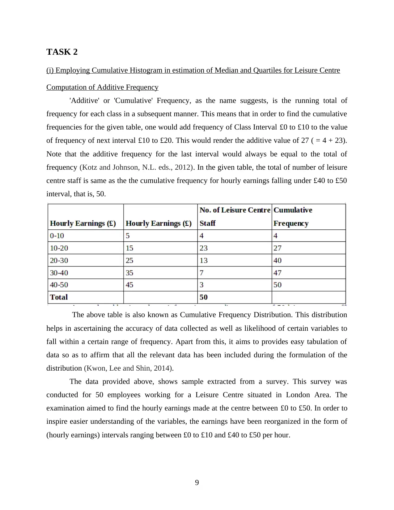
'Additive' or 'Cumulative' Frequency, as the name suggests, is the running total of
frequency for each class in a subsequent manner. This means that in order to find the cumulative
frequencies for the given table, one would add frequency of Class Interval £0 to £10 to the value
of frequency of next interval £10 to £20. This would render the additive value of 27 ( = 4 + 23).
Note that the additive frequency for the last interval would always be equal to the total of
frequency (Kotz and Johnson, N.L. eds., 2012). In the given table, the total of number of leisure
centre staff is same as the the cumulative frequency for hourly earnings falling under £40 to £50
interval, that is, 50.
The above table is also known as Cumulative Frequency Distribution. This distribution
helps in ascertaining the accuracy of data collected as well as likelihood of certain variables to
fall within a certain range of frequency. Apart from this, it aims to provides easy tabulation of
data so as to affirm that all the relevant data has been included during the formulation of the
distribution (Kwon, Lee and Shin, 2014).
The data provided above, shows sample extracted from a survey. This survey was
conducted for 50 employees working for a Leisure Centre situated in London Area. The
examination aimed to find the hourly earnings made at the centre between £0 to £50. In order to
inspire easier understanding of the variables, the earnings have been reorganized in the form of
(hourly earnings) intervals ranging between £0 to £10 and £40 to £50 per hour.
9
(i) Employing Cumulative Histogram in estimation of Median and Quartiles for Leisure Centre
Computation of Additive Frequency
'Additive' or 'Cumulative' Frequency, as the name suggests, is the running total of
frequency for each class in a subsequent manner. This means that in order to find the cumulative
frequencies for the given table, one would add frequency of Class Interval £0 to £10 to the value
of frequency of next interval £10 to £20. This would render the additive value of 27 ( = 4 + 23).
Note that the additive frequency for the last interval would always be equal to the total of
frequency (Kotz and Johnson, N.L. eds., 2012). In the given table, the total of number of leisure
centre staff is same as the the cumulative frequency for hourly earnings falling under £40 to £50
interval, that is, 50.
The above table is also known as Cumulative Frequency Distribution. This distribution
helps in ascertaining the accuracy of data collected as well as likelihood of certain variables to
fall within a certain range of frequency. Apart from this, it aims to provides easy tabulation of
data so as to affirm that all the relevant data has been included during the formulation of the
distribution (Kwon, Lee and Shin, 2014).
The data provided above, shows sample extracted from a survey. This survey was
conducted for 50 employees working for a Leisure Centre situated in London Area. The
examination aimed to find the hourly earnings made at the centre between £0 to £50. In order to
inspire easier understanding of the variables, the earnings have been reorganized in the form of
(hourly earnings) intervals ranging between £0 to £10 and £40 to £50 per hour.
9
Ogive
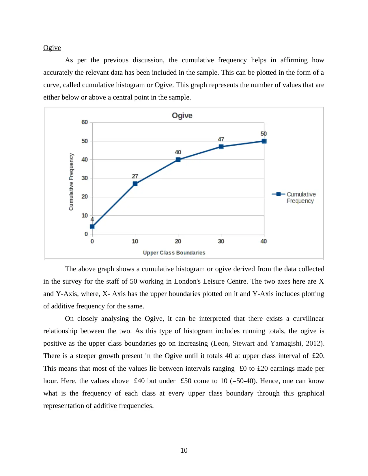
As per the previous discussion, the cumulative frequency helps in affirming how
accurately the relevant data has been included in the sample. This can be plotted in the form of a
curve, called cumulative histogram or Ogive. This graph represents the number of values that are
either below or above a central point in the sample.
The above graph shows a cumulative histogram or ogive derived from the data collected
in the survey for the staff of 50 working in London's Leisure Centre. The two axes here are X
and Y-Axis, where, X- Axis has the upper boundaries plotted on it and Y-Axis includes plotting
of additive frequency for the same.
On closely analysing the Ogive, it can be interpreted that there exists a curvilinear
relationship between the two. As this type of histogram includes running totals, the ogive is
positive as the upper class boundaries go on increasing (Leon, Stewart and Yamagishi, 2012).
There is a steeper growth present in the Ogive until it totals 40 at upper class interval of £20.
This means that most of the values lie between intervals ranging £0 to £20 earnings made per
hour. Here, the values above £40 but under £50 come to 10 (=50-40). Hence, one can know
what is the frequency of each class at every upper class boundary through this graphical
representation of additive frequencies.
10
⊘ This is a preview!⊘
Do you want full access?
Subscribe today to unlock all pages.
Trusted by 1+ million students worldwide
1 out of 23
Related Documents


Your All-in-One AI-Powered Toolkit for Academic Success.
+13062052269
info@desklib.com
Available 24*7 on WhatsApp / Email
![[object Object]](/_next/static/media/star-bottom.7253800d.svg)
Unlock your academic potential
Copyright © 2020–2026 A2Z Services. All Rights Reserved. Developed and managed by ZUCOL.