Statistics for Managerial Decisions: Data Analysis and Interpretation

This statistics assignment covers various statistical concepts and their applications in managerial decision-making. The assignment includes solutions to problems involving stem-leaf plots, histograms, market capitalization analysis, numerical statistics, box-whisker plots, probability calculations (including Poisson and normal distributions), and normal probability plots. The analysis encompasses topics like stock valuation, rental data comparison across cities, crop yield probabilities, and rainfall patterns. The assignment also includes the computation and interpretation of confidence intervals for different variables, assessing their utility in differentiating patient categories based on serum cholesterol, resting blood pressure, OLDPEAK, and maximum heart rate achieved. Excel is used to facilitate calculations, with relevant outputs provided to support the analysis and interpretations.

STATISTICS FOR MANGERIAL DECISIONS
STUDENT iD:
[Pick the date]

Question 1
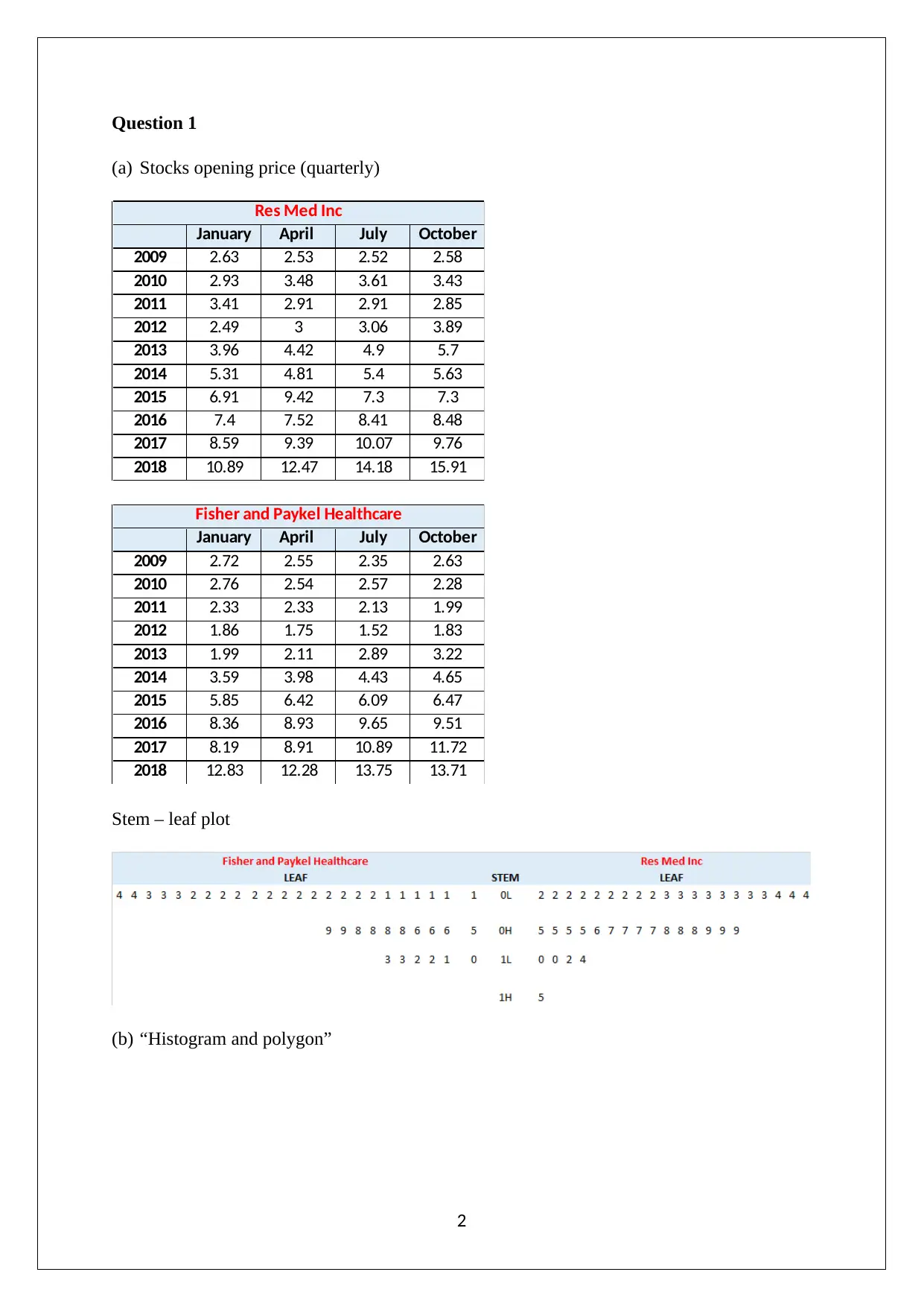
(a) Stocks opening price (quarterly)
January April July October
2009 2.63 2.53 2.52 2.58
2010 2.93 3.48 3.61 3.43
2011 3.41 2.91 2.91 2.85
2012 2.49 3 3.06 3.89
2013 3.96 4.42 4.9 5.7
2014 5.31 4.81 5.4 5.63
2015 6.91 9.42 7.3 7.3
2016 7.4 7.52 8.41 8.48
2017 8.59 9.39 10.07 9.76
2018 10.89 12.47 14.18 15.91
Res Med Inc
January April July October
2009 2.72 2.55 2.35 2.63
2010 2.76 2.54 2.57 2.28
2011 2.33 2.33 2.13 1.99
2012 1.86 1.75 1.52 1.83
2013 1.99 2.11 2.89 3.22
2014 3.59 3.98 4.43 4.65
2015 5.85 6.42 6.09 6.47
2016 8.36 8.93 9.65 9.51
2017 8.19 8.91 10.89 11.72
2018 12.83 12.28 13.75 13.71
Fisher and Paykel Healthcare
Stem – leaf plot
(b) “Histogram and polygon”
2

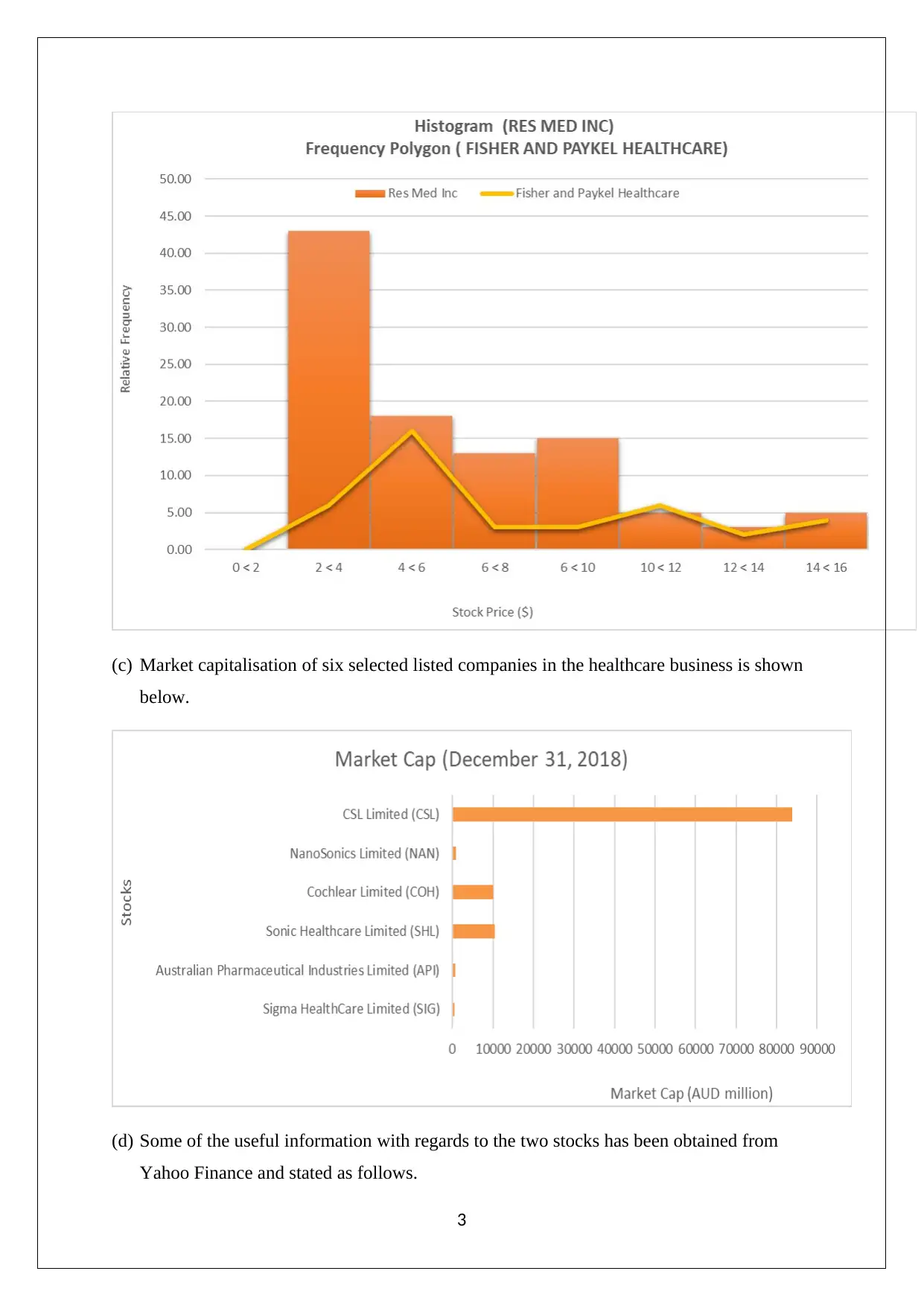
(c) Market capitalisation of six selected listed companies in the healthcare business is shown
below.
(d) Some of the useful information with regards to the two stocks has been obtained from
Yahoo Finance and stated as follows.
3

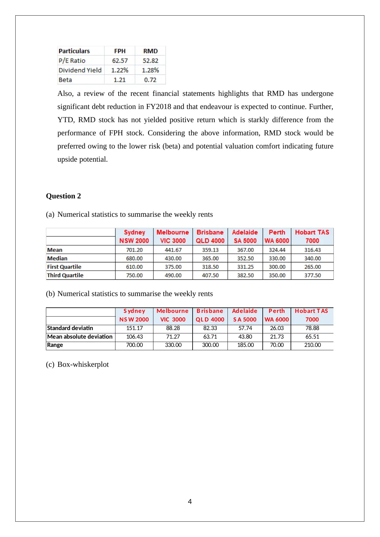
Also, a review of the recent financial statements highlights that RMD has undergone
significant debt reduction in FY2018 and that endeavour is expected to continue. Further,
YTD, RMD stock has not yielded positive return which is starkly difference from the
performance of FPH stock. Considering the above information, RMD stock would be
preferred owing to the lower risk (beta) and potential valuation comfort indicating future
upside potential.
Question 2
(a) Numerical statistics to summarise the weekly rents
(b) Numerical statistics to summarise the weekly rents
Standard deviatin 151.17 88.28 82.33 57.74 26.03 78.88
Mean absolute deviation 106.43 71.27 63.71 43.80 21.73 65.51
Range 700.00 330.00 300.00 185.00 70.00 210.00
H obart T AS
7000
S ydney
NS W 2000
Melbourne
VIC 3000
B ris bane
Q L D 4000
Adelaide
S A 5000
P erth
WA 6000
(c) Box-whiskerplot
4

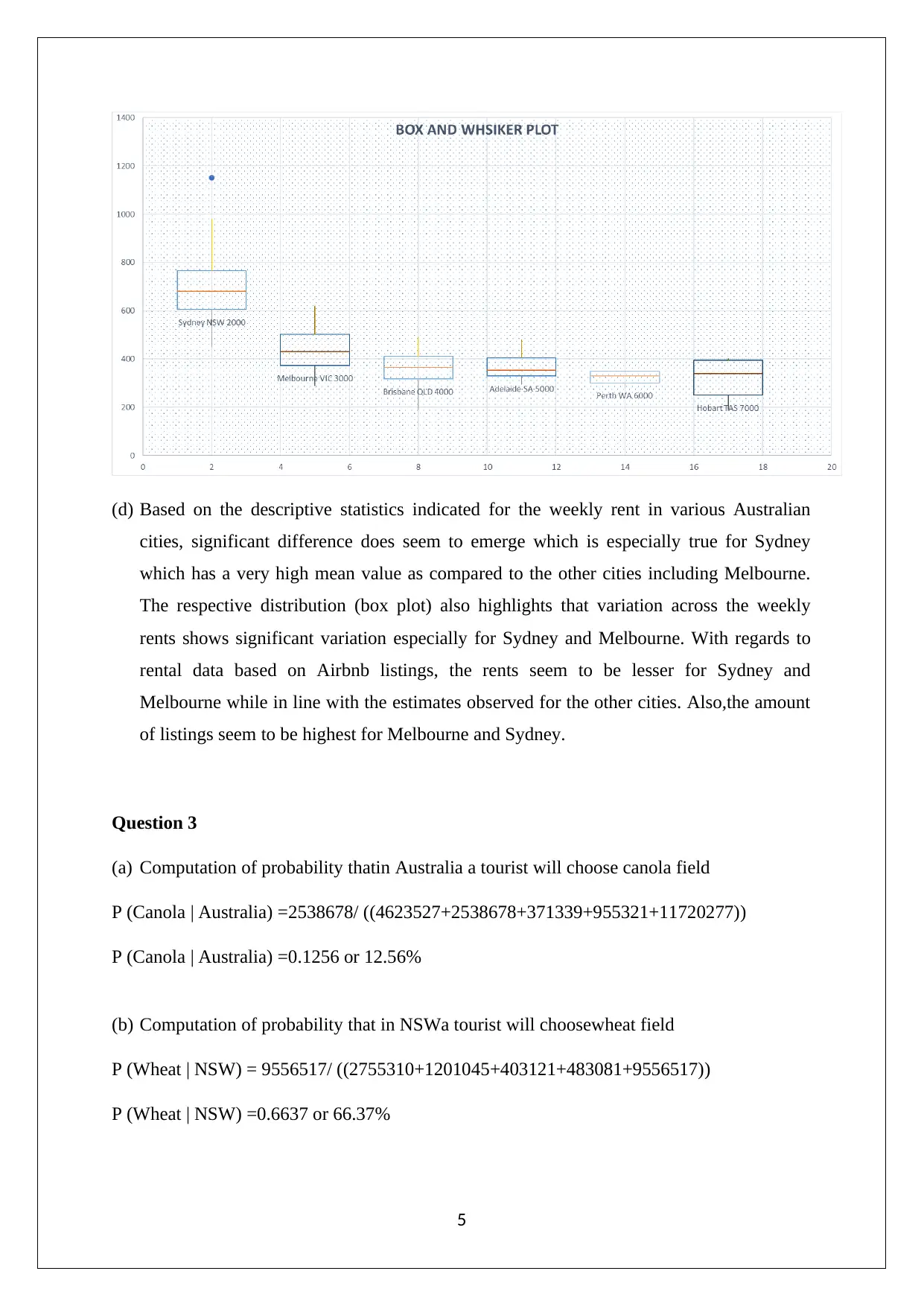
(d) Based on the descriptive statistics indicated for the weekly rent in various Australian
cities, significant difference does seem to emerge which is especially true for Sydney
which has a very high mean value as compared to the other cities including Melbourne.
The respective distribution (box plot) also highlights that variation across the weekly
rents shows significant variation especially for Sydney and Melbourne. With regards to
rental data based on Airbnb listings, the rents seem to be lesser for Sydney and
Melbourne while in line with the estimates observed for the other cities. Also,the amount
of listings seem to be highest for Melbourne and Sydney.
Question 3
(a) Computation of probability thatin Australia a tourist will choose canola field
P (Canola | Australia) =2538678/ ((4623527+2538678+371339+955321+11720277))
P (Canola | Australia) =0.1256 or 12.56%
(b) Computation of probability that in NSWa tourist will choosewheat field
P (Wheat | NSW) = 9556517/ ((2755310+1201045+403121+483081+9556517))
P (Wheat | NSW) =0.6637 or 66.37%
5

(c) Yield of crop =Production of crop /Area of filed
Barley yield (NSW)=Production/Area=2755310/1008269=2.733
Barley yield (VIC)=Production/Area= (3100466)/954176=3.249
Barley yield (QID)=Production/Area=413023/141960=2.909
Barley yield (SA)=Production/Area=2744507/922787=2.974
P (Barley | SA) = 2.974 / (2.733 + 3.249 + 2.909 + 2.974) = 0.251 or 25.1%
(d) Considering that a relative standard error in excess of 50% is witnessed for the grain
sorghum estimates in the state of South Australia, hence these estimates would be termed
as unreliable as per ABS.
Question 4
(a) Rainfall = Poisson distribution
6

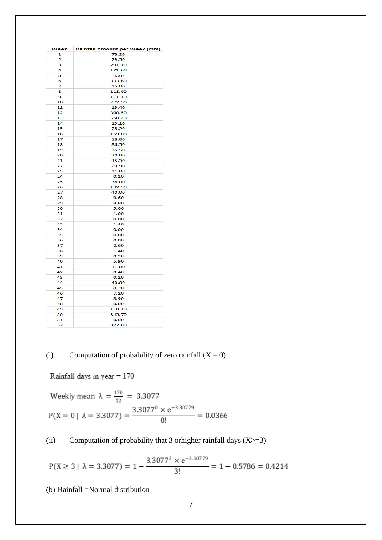
(i) Computation of probability of zero rainfall (X = 0)
(ii) Computation of probability that 3 orhigher rainfall days (X>=3)
(b) Rainfall =Normal distribution
7

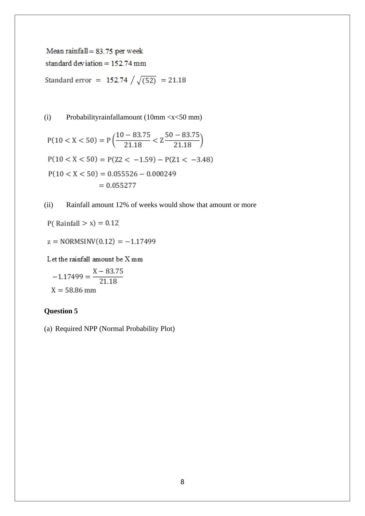
(i) Probabilityrainfallamount (10mm <x<50 mm)
(ii) Rainfall amount 12% of weeks would show that amount or more
Question 5
(a) Required NPP (Normal Probability Plot)
8

Interpretation: The normal probability plot is a tool which can be used to comment on
whether the normal distribution would be a suitable fit for the underlying variable or not. The
key aspect to be noted is the shape of the plot. The resting blood pressure variable seems to
have a linear trend which would signify the suitability of normal distribution for the fit of the
above variable.
9

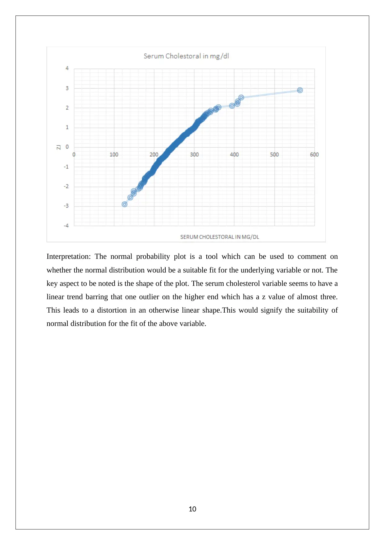
Interpretation: The normal probability plot is a tool which can be used to comment on
whether the normal distribution would be a suitable fit for the underlying variable or not. The
key aspect to be noted is the shape of the plot. The serum cholesterol variable seems to have a
linear trend barring that one outlier on the higher end which has a z value of almost three.
This leads to a distortion in an otherwise linear shape.This would signify the suitability of
normal distribution for the fit of the above variable.
10

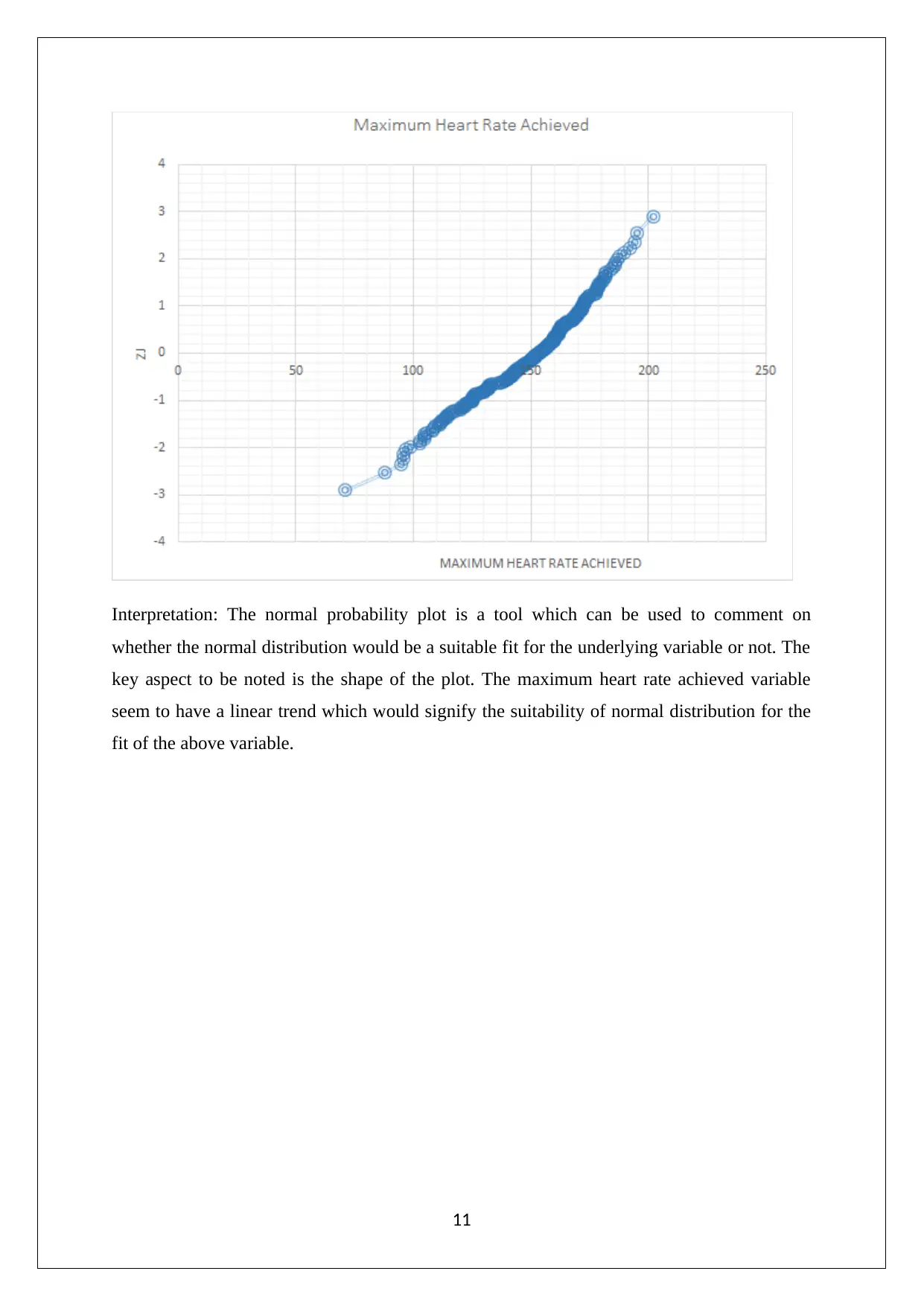
Interpretation: The normal probability plot is a tool which can be used to comment on
whether the normal distribution would be a suitable fit for the underlying variable or not. The
key aspect to be noted is the shape of the plot. The maximum heart rate achieved variable
seem to have a linear trend which would signify the suitability of normal distribution for the
fit of the above variable.
11

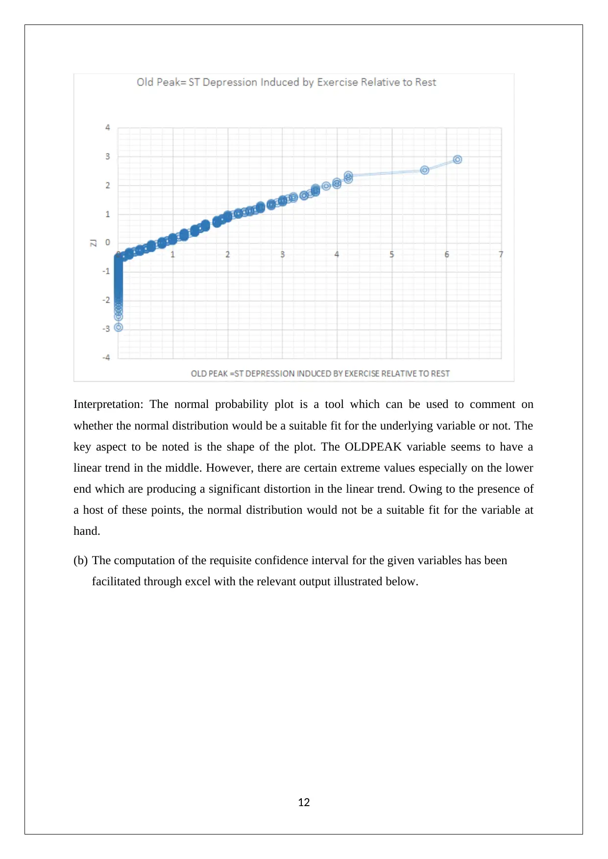
Interpretation: The normal probability plot is a tool which can be used to comment on
whether the normal distribution would be a suitable fit for the underlying variable or not. The
key aspect to be noted is the shape of the plot. The OLDPEAK variable seems to have a
linear trend in the middle. However, there are certain extreme values especially on the lower
end which are producing a significant distortion in the linear trend. Owing to the presence of
a host of these points, the normal distribution would not be a suitable fit for the variable at
hand.
(b) The computation of the requisite confidence interval for the given variables has been
facilitated through excel with the relevant output illustrated below.
12