Statistics and Probability Homework - Covariance and Hypothesis

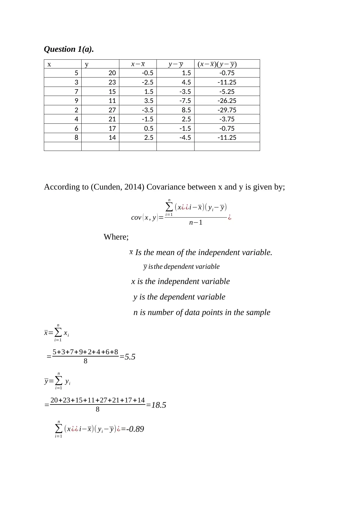
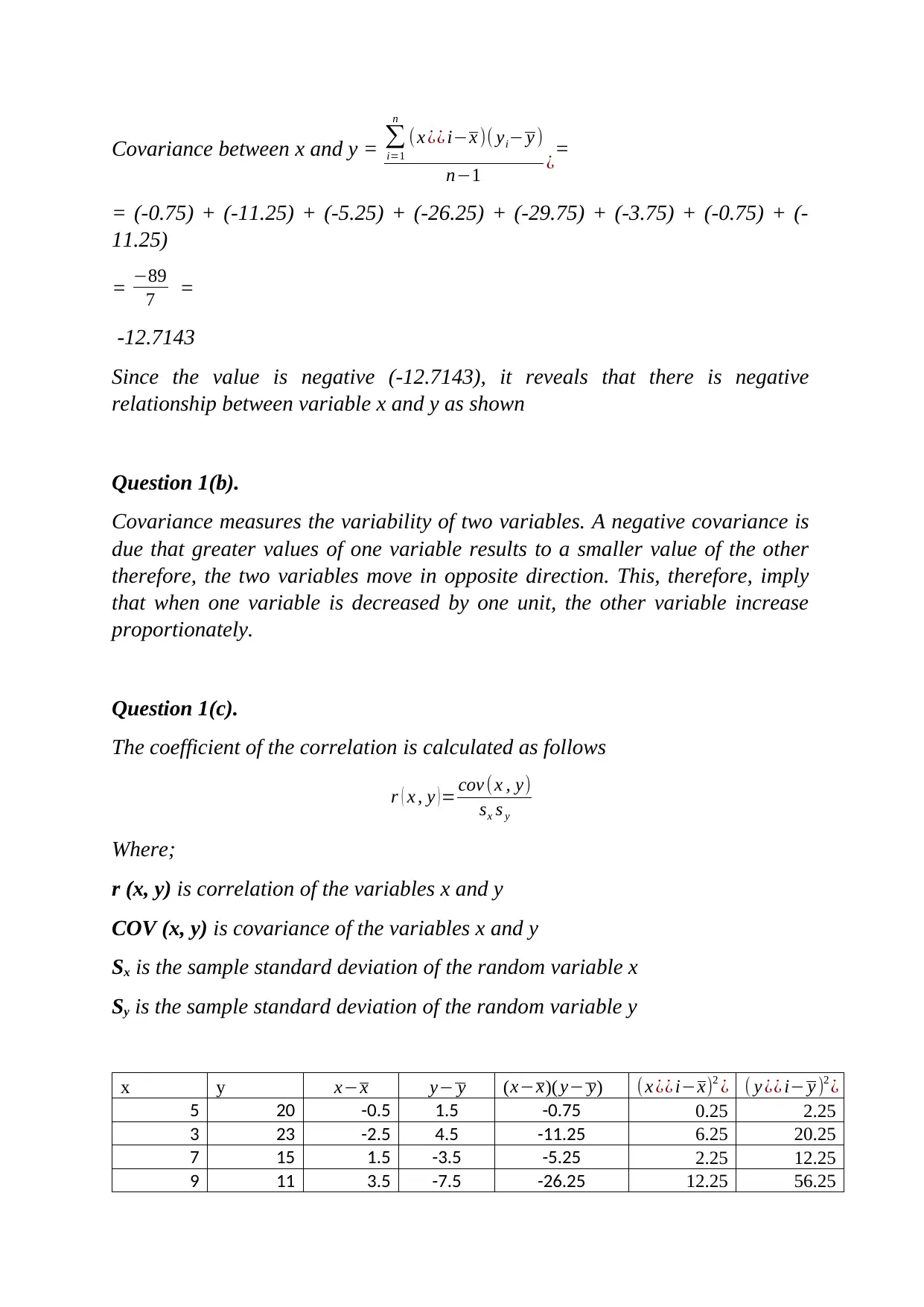
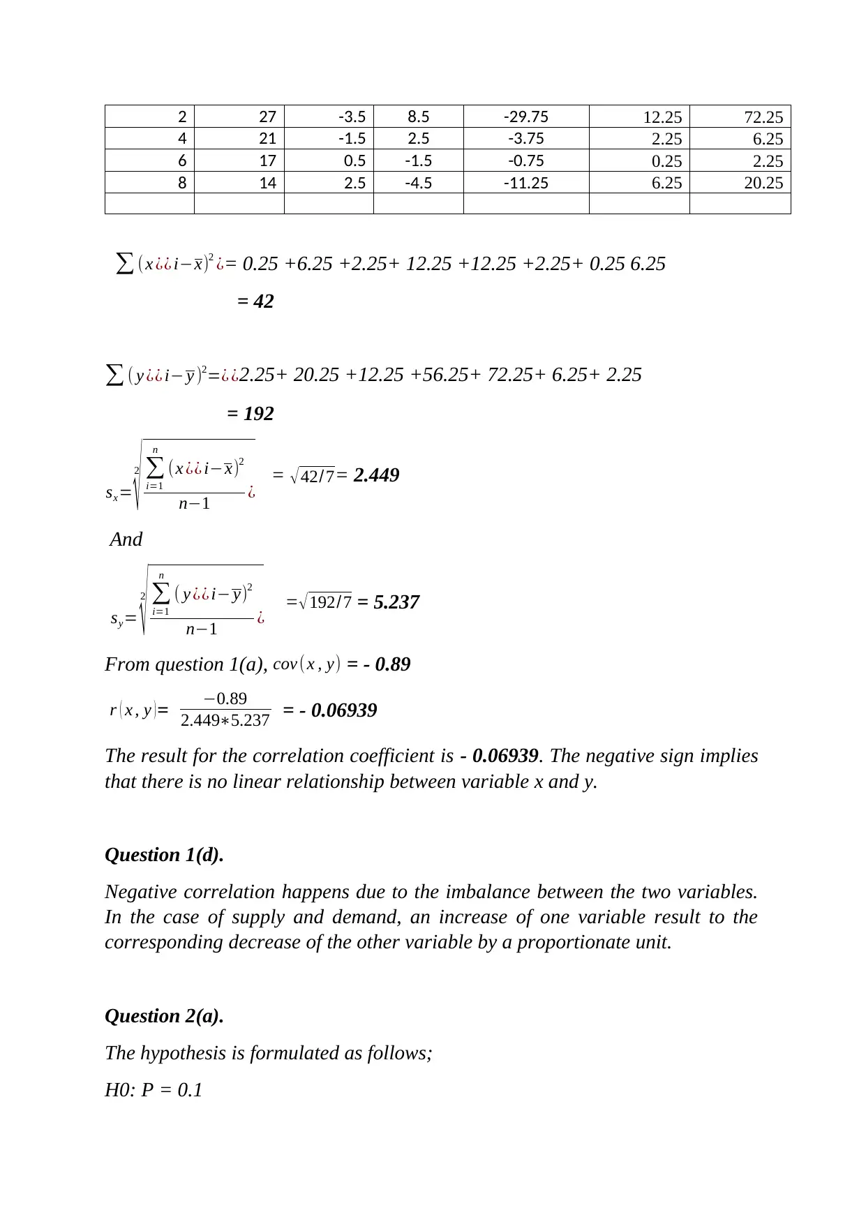
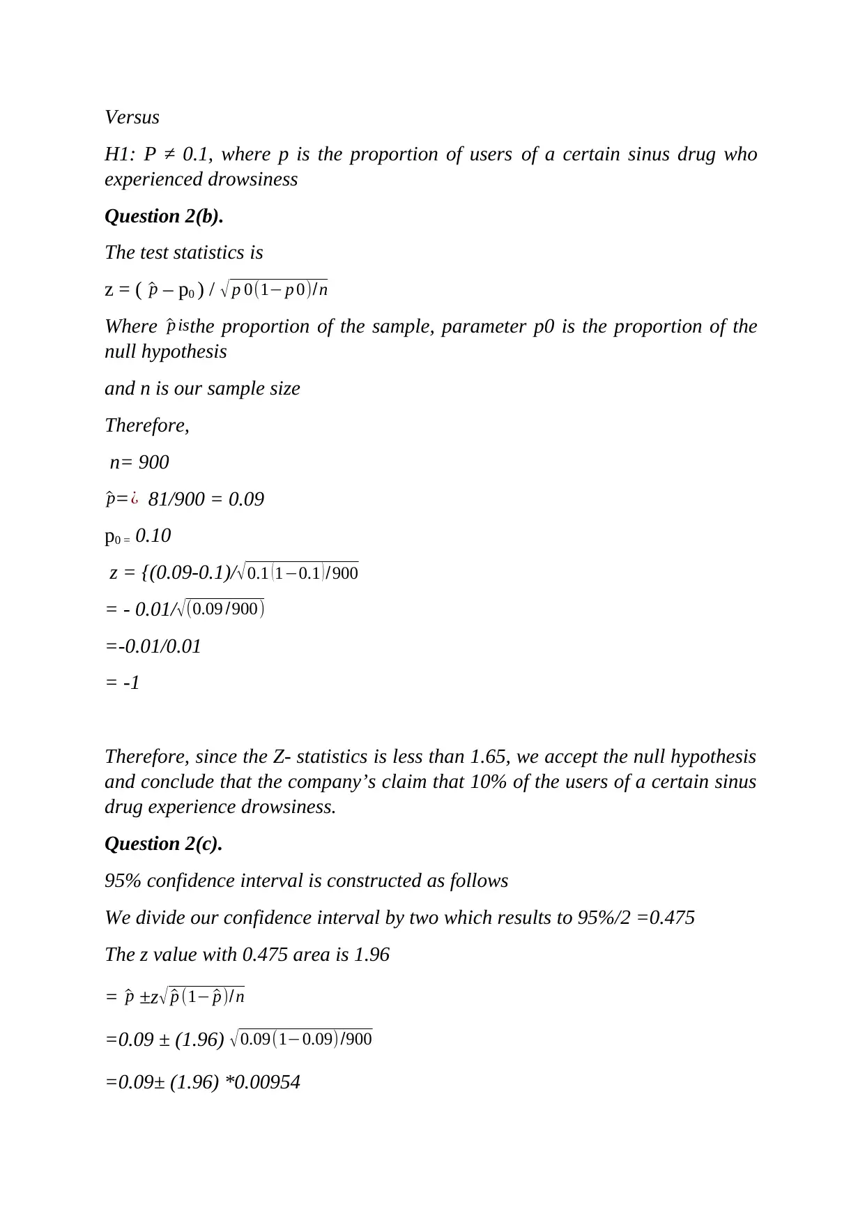
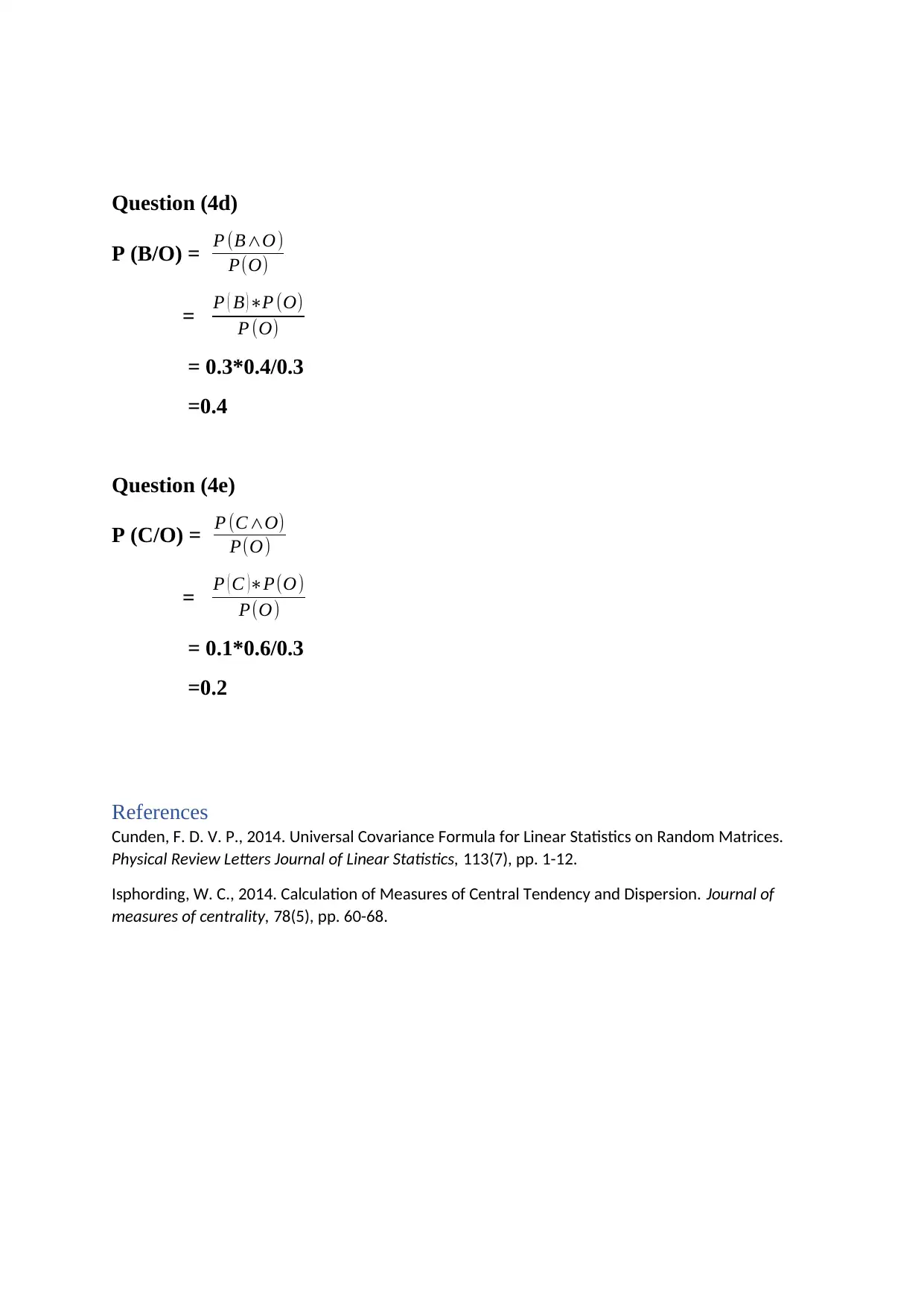
This homework assignment presents a comprehensive analysis of statistical concepts. It begins with calculating covariance and correlation coefficients between two variables, interpreting their relationship, and discussing the implications of negative correlation. The assignment then delves into hypothesis testing, formulating null and alternative hypotheses, calculating test statistics, and constructing confidence intervals to assess the validity of a claim. Further, the solution explores measures of central tendency (mean, median, and mode), their agreement, and the impact of outliers. Finally, it concludes with probability calculations using a tree diagram to determine conditional probabilities. The assignment uses real-world data and provides detailed calculations and interpretations, referencing relevant statistical concepts and formulas.

Question 1(a).
x y x−x y− y ( x−x)( y− y)
5 20 -0.5 1.5 -0.75
3 23 -2.5 4.5 -11.25
7 15 1.5 -3.5 -5.25
9 11 3.5 -7.5 -26.25
2 27 -3.5 8.5 -29.75
4 21 -1.5 2.5 -3.75
6 17 0.5 -1.5 -0.75
8 14 2.5 -4.5 -11.25
According to (Cunden, 2014) Covariance between x and y is given by;
cov ( x , y ) =
∑
i=1
n
( x¿ ¿i−x)( yi− y)
n−1 ¿
Where;
x Is the mean of the independent variable.
y isthe dependent variable
x is the independent variable
y is the dependent variable
n is number of data points in the sample
x=∑
i=1
n
xi
= 5+3+7+ 9+ 2+ 4 +6+8
8 =5.5
y=∑
i=1
n
yi
= 20+23+15+11+27+21+17 +14
8 =18.5
∑
i=1
n
(x ¿¿ i−x)( yi − y)¿=-0.89

Covariance between x and y = ∑
i=1
n
(x ¿¿ i−x )( yi− y )
n−1 ¿=
= (-0.75) + (-11.25) + (-5.25) + (-26.25) + (-29.75) + (-3.75) + (-0.75) + (-
11.25)
= −89
7 =
-12.7143
Since the value is negative (-12.7143), it reveals that there is negative
relationship between variable x and y as shown
Question 1(b).
Covariance measures the variability of two variables. A negative covariance is
due that greater values of one variable results to a smaller value of the other
therefore, the two variables move in opposite direction. This, therefore, imply
that when one variable is decreased by one unit, the other variable increase
proportionately.
Question 1(c).
The coefficient of the correlation is calculated as follows
r ( x , y )= cov ( x , y)
sx s y
Where;
r (x, y) is correlation of the variables x and y
COV (x, y) is covariance of the variables x and y
Sx is the sample standard deviation of the random variable x
Sy is the sample standard deviation of the random variable y
x y x−x y− y ( x−x)( y− y) (x ¿¿ i−x)2 ¿ ( y ¿¿ i− y )2 ¿
5 20 -0.5 1.5 -0.75 0.25 2.25
3 23 -2.5 4.5 -11.25 6.25 20.25
7 15 1.5 -3.5 -5.25 2.25 12.25
9 11 3.5 -7.5 -26.25 12.25 56.25

2 27 -3.5 8.5 -29.75 12.25 72.25
4 21 -1.5 2.5 -3.75 2.25 6.25
6 17 0.5 -1.5 -0.75 0.25 2.25
8 14 2.5 -4.5 -11.25 6.25 20.25
∑ (x ¿¿ i−x)2 ¿= 0.25 +6.25 +2.25+ 12.25 +12.25 +2.25+ 0.25 6.25
= 42
∑ ( y ¿¿ i− y )2=¿ ¿2.25+ 20.25 +12.25 +56.25+ 72.25+ 6.25+ 2.25
= 192
sx=
2
√ ∑
i=1
n
(x ¿¿ i−x)2
n−1 ¿ = √42/ 7= 2.449
And
sy=
2
√ ∑
i=1
n
( y ¿¿ i− y)2
n−1 ¿ =√192/7 = 5.237
From question 1(a), cov (x , y) = - 0.89
r ( x , y )= −0.89
2.449∗5.237 = - 0.06939
The result for the correlation coefficient is - 0.06939. The negative sign implies
that there is no linear relationship between variable x and y.
Question 1(d).
Negative correlation happens due to the imbalance between the two variables.
In the case of supply and demand, an increase of one variable result to the
corresponding decrease of the other variable by a proportionate unit.
Question 2(a).
The hypothesis is formulated as follows;
H0: P = 0.1

Versus
H1: P ≠ 0.1, where p is the proportion of users of a certain sinus drug who
experienced drowsiness
Question 2(b).
The test statistics is
z = ( ^p – p0 ) / √ p 0(1− p 0)/n
Where ^p isthe proportion of the sample, parameter p0 is the proportion of the
null hypothesis
and n is our sample size
Therefore,
n= 900
^p=¿ 81/900 = 0.09
p0 = 0.10
z = {(0.09-0.1)/ √ 0.1 ( 1−0.1 ) /900
= - 0.01/√(0.09 /900)
=-0.01/0.01
= -1
Therefore, since the Z- statistics is less than 1.65, we accept the null hypothesis
and conclude that the company’s claim that 10% of the users of a certain sinus
drug experience drowsiness.
Question 2(c).
95% confidence interval is constructed as follows
We divide our confidence interval by two which results to 95%/2 =0.475
The z value with 0.475 area is 1.96
= ^p ±z√ ^p (1− ^p)/n
=0.09 ± (1.96) √0.09(1−0.09)/900
=0.09± (1.96) *0.00954

=0.09±0.01870
The lower confidence interval for the proportion is 0.0713
The upper confidence interval for the proportion is 0.1087
Question 2(d).
Our sample result is as calculated; 81/900 = 0.09, which falls between 0.0713
and 0.1087. Since this is true, we do not reject the null hypothesis
Question 3(a).
sum = 730 + 730 + 730 + 930 + 700 + 570 + 690 + 1,030 + 740 + 620 + 720
+ 670 +560 + 740 + 650 + 660 +850 +930 + 600 + 620 +760+ 690 + 710
+ 500 +730 + 800+ 820+ 840+ 720+ 700
= 18,850
Mean = ∑ x/n
= 18,850/30
= 628.3333333
median
To calculate the median, we arrange the data in ascending order (Isphording,
2014) and at the same time eliminate the numbers that are repeated
730, 500, 560, 570, 600, 620, 650, 660, 670, 690, 690, 700, 710, 720, 730, 740,
760, 820, 840, 850, 930, 1,030, 620, 730, 740, 800.
= (710+720)/2
= 1430/2
=715
Median is 715
Mode is the most repeated number in the data.
From our data
730,500, 560, 570, 600, 620, 650, 660, 670, 690, 690, 700, 700, 710, 720, 720,
730, 730, 740, 760, 820, 840, 850, 930, 930, 1,030, 620, 730, 740, 800.

The mode is 730 which is repeated thrice
Question 3(b).
The value of mean, median and mode is 628.33,715,730 respectively
Therefore, the three measures of central tendency do not agree because of the
existence of extreme values bringing in about the issue of outliers.
Question 3(c).
Standard deviation is calculated as follows;
The mean of the data is 628.33
x (x-628.33) (x-628.33) ^2
730 101.67 10,336.11
690 61.67 3,802.78
560 -68.33 4,669.44
600 -28.33 802.78
730 101.67 10,336.11
730 101.67 10,336.79
1030 401.67 161,336.11
740 111.67 12,470.19
620 8.33 69.39
800 171.67 29,470.59
730 101.67 10,336.11
740 111.67 12,469.44
650 21.67 469.44
760 131.67 17,336.11
820 191.67 36,736.11
930 301.67 91,002.78
620 -8.33 69.44
660 31.67 1,002.78
690 61.67 3,802.78
840 211.67 44,802.78
700 71.67 5,136.11
720 91.67 8,402.78
850 221.67 49,136.11

710 81.67 6,669.44
720 91.67 8,402.78
570 -58.33 3,402.78
670 41.67 1,736.11
930 301.67 91,002.78
500 -128.33 16,469.44
700 71.67 5,136.11
Standard deviation is;
¿ 2
√ ∑ (x −x¿¿)2 ¿ ¿/n
=10,336.11 + 3,802.78 + 4,669.44 + 802.78 +10,336.11+ 10,336.79 +
161,336.11+ 12,470.19 + 69.39 + 29,470.59 + 10,336.11 + 12,469.44 +
469.44 + 17,336.11 + 36,736.11+ 91,002.78 + 69.44 + 1,002.78 + 3,802.78 +
44,802.78 + 5,136.11 + 8,402.78 + 49,136.11 + 6,669.44 + 8,402.78 +
3,402.78 + 1,736.11 + 91,002.78 + 16,469.44 + 5,136.11
= 657,152.51
= √657,152.51/30
= √21,905.08
= 148
Question 3(d).
Yes, there are outliers in the data.
Question 3(e).
Empirical rule states that data can be identified to be from a normal distribution
if
Mean=median=mode
From the data, mean= 628.33, media= 715, mode=730 which reveal that the
data were not obtained from the normal distribution.

Question (4a)
Below is a tree diagram describing the probabilities
P (A) = 0.6
P (0) = 0.8
P (A) and P (0) is given by P (A) * P (0)
=0.6*0.8
=0.48
Question (4b)
P (O) =P (OA) + P (OB) + P (OC)
= (0.8*0.6) + (0.6*0.3) + (0.1*0.4)
=0.7
Question (4c)
P (A/O) = P ¿ ¿
= 0.48/0.7
=0.4

Question (4d)
P (B/O) = P (B∧O)
P(O)
= P ( B )∗P (O)
P (O)
= 0.3*0.4/0.3
=0.4
Question (4e)
P (C/O) = P (C∧O)
P(O)
= P ( C )∗P(O)
P(O)
= 0.1*0.6/0.3
=0.2
References
Cunden, F. D. V. P., 2014. Universal Covariance Formula for Linear Statistics on Random Matrices.
Physical Review Letters Journal of Linear Statistics, 113(7), pp. 1-12.
Isphording, W. C., 2014. Calculation of Measures of Central Tendency and Dispersion. Journal of
measures of centrality, 78(5), pp. 60-68.