Statistics Assignment Solution: Probability, Hypothesis Testing, & CI

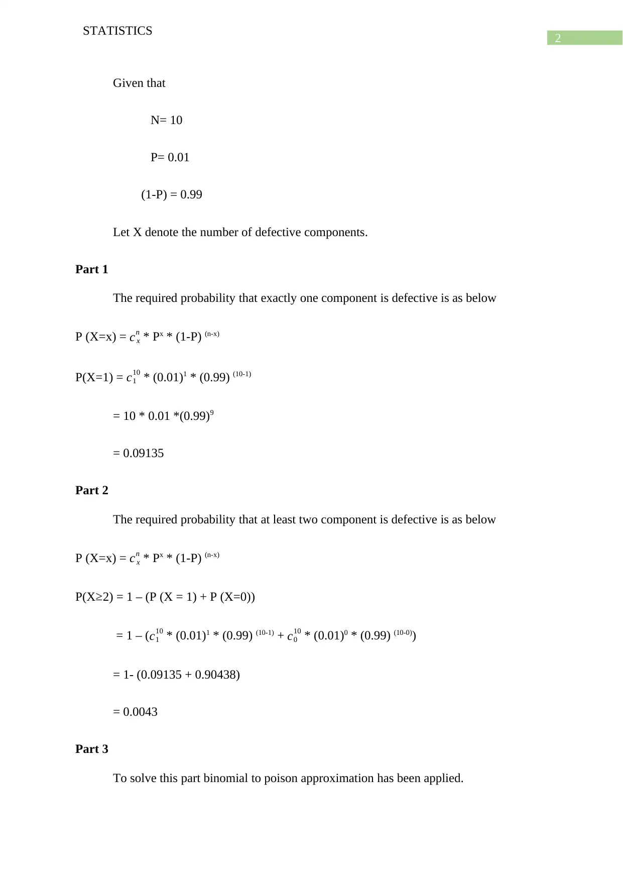
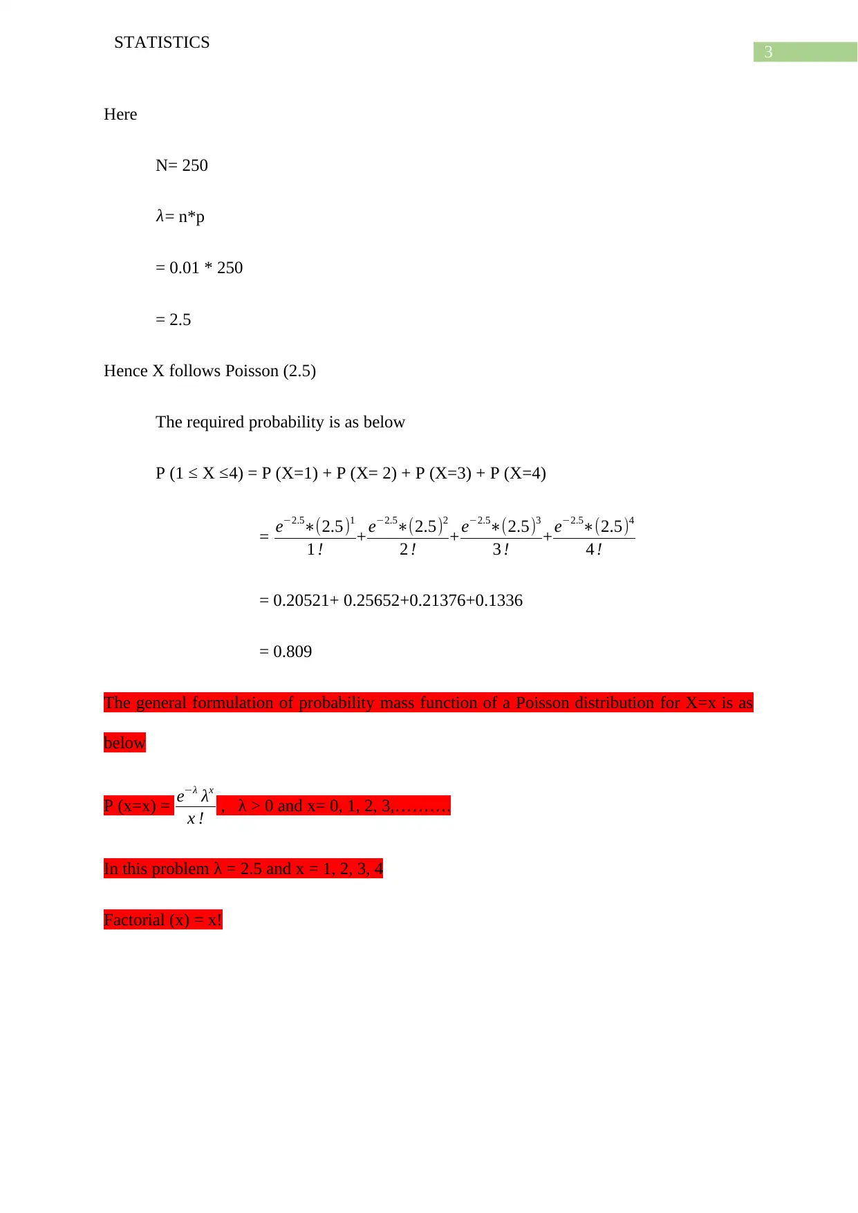
This statistics assignment solution addresses problems involving probability distributions, hypothesis testing, and confidence intervals. The assignment begins with calculating probabilities using the binomial distribution, including finding the probability of exactly one defective component and at least two defective components in a box. It then applies a Poisson approximation to solve a probability problem for a larger batch of components. The second part of the assignment focuses on hypothesis testing using a chi-square test to determine if there's a difference in customer brand preference across different supermarkets. Finally, it calculates a 95% confidence interval for the true mean rent and determines the required sample size for a specified margin of error.

Running head: STATISTICS
Statistics
Name of the Student:
Name of the University:
Author note:

1
STATISTICS
Table of Contents
Answer to the question 1............................................................................................................2
Part 1......................................................................................................................................2
Part 2......................................................................................................................................2
Part 3......................................................................................................................................2
Answer to the question 2............................................................................................................3
Part (a)....................................................................................................................................3
Part (b)....................................................................................................................................5
Bibliography...............................................................................................................................6
Answer to the question 1

2
STATISTICS
Given that
N= 10
P= 0.01
(1-P) = 0.99
Let X denote the number of defective components.
Part 1
The required probability that exactly one component is defective is as below
P (X=x) = c x
n * Px * (1-P) (n-x)
P(X=1) = c1
10 * (0.01)1 * (0.99) (10-1)
= 10 * 0.01 *(0.99)9
= 0.09135
Part 2
The required probability that at least two component is defective is as below
P (X=x) = c x
n * Px * (1-P) (n-x)
P(X ≥2) = 1 – (P (X = 1) + P (X=0))
= 1 – ( c1
10 * (0.01)1 * (0.99) (10-1) + c0
10 * (0.01)0 * (0.99) (10-0))
= 1- (0.09135 + 0.90438)
= 0.0043
Part 3
To solve this part binomial to poison approximation has been applied.

3
STATISTICS
Here
N= 250
λ= n*p
= 0.01 * 250
= 2.5
Hence X follows Poisson (2.5)
The required probability is as below
P (1 ≤ X ≤4) = P (X=1) + P (X= 2) + P (X=3) + P (X=4)
= e−2.5∗(2.5)1
1 ! + e−2.5∗(2.5)2
2 ! + e−2.5∗(2.5)3
3 ! + e−2.5∗(2.5)4
4 !
= 0.20521+ 0.25652+0.21376+0.1336
= 0.809
The general formulation of probability mass function of a Poisson distribution for X=x is as
below
P (x=x) = e−λ λx
x ! , λ > 0 and x= 0, 1, 2, 3,……….
In this problem λ = 2.5 and x = 1, 2, 3, 4
Factorial (x) = x!

4
STATISTICS
Answer to the question 2
Part (a)
Null hypothesis: There is no differences on the customers brand preference among the
different super market.
Alternative hypothesis: There is a differences on the customers brand preference among the
different super market.
Table 1 Observe Frequency
Table 2 Expected Frequency
Table 3 Test statistic
Chi- square test statistic is as below

5
STATISTICS
Χ2 =∑ ( Oi , j−Ei , j)2
Ei , j
, i = 1, 2, 3 and j= 1, 2
Test statistic = 6.47
Degrees of freedom = (3-1) * (2-1)
= 2
Critical value = 0.039
Alpha = 0.05 (at 5%)
It has been seen that critical value < alpha. Hence the null hypothesis of this test is
significant and at the same time the alternative hypothesis is accepted. Thus it may be
summarised that there is a differences on the customers brand preference among the different
super market.
Part (b)
Given that
N= 60
Mean = 1000
Standard deviation = 200
The 95% confidence interval is as below
Mean ±1.96 * standard deviation
√ (n)
= 1000 ±1.96 * 200
√(60)
= (949.39, 1050.61)

6
STATISTICS
Hence at 95% the true mean rent is lies between € 949.39 and € 1050.61.
Again
Multiple of Z at 90% = 1.645
50 = 1.645 * 200
√(n)
Sqrt (n) = 329
50
Sqrt (n) = 6.58
n = 43.3
Therefore the required sample size = 44
Bibliography
Daskalakis, C., Diakonikolas, I. and Servedio, R.A., 2015. Learning poisson binomial
distributions. Algorithmica, 72(1), pp.316-357.
Hong, Y., 2013. On computing the distribution function for the Poisson binomial distribution.
Computational Statistics & Data Analysis, 59, pp.41-51.
Lee, D.K., 2016. Alternatives to P value: confidence interval and effect size. Korean journal
of anesthesiology, 69(6), p.555.
McHugh, M.L., 2013. The chi-square test of independence. Biochemia medica: Biochemia
medica, 23(2), pp.143-149.

7
STATISTICS
McHugh, M.L., 2013. The chi-square test of independence. Biochemia medica: Biochemia
medica, 23(2), pp.143-149.
Moinester, M. and Gottfried, R., 2014. Sample size estimation for correlations with pre-
specified confidence interval. The quantitative methods for psychology, 10(2), pp.124-130.