Analytical Methods for Engineers: Statistics & Probability TMA 4

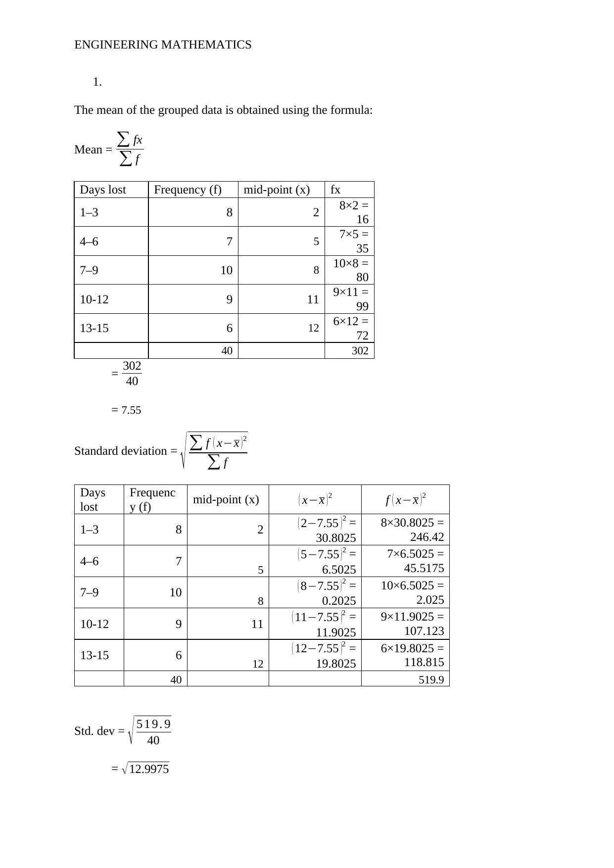
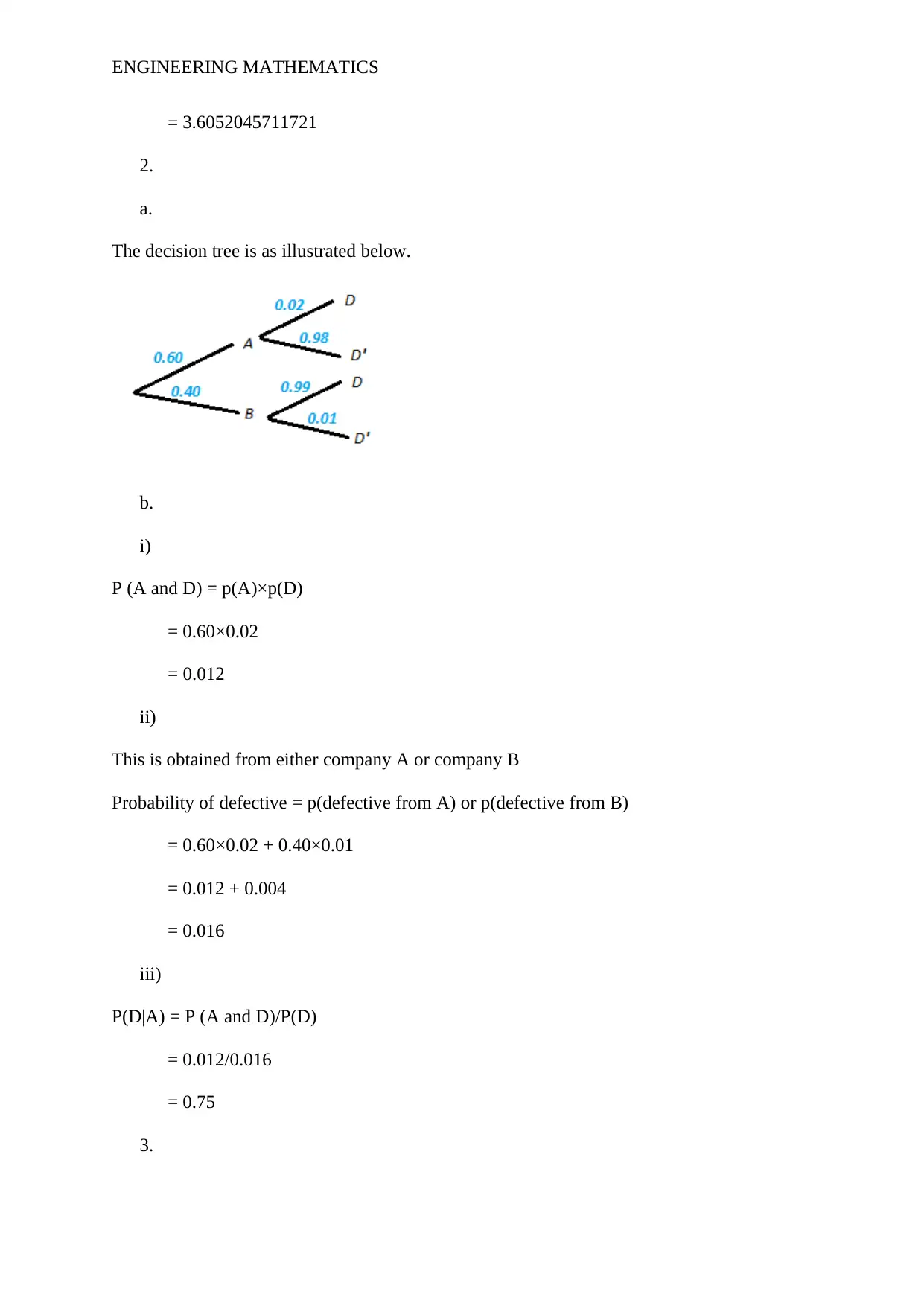
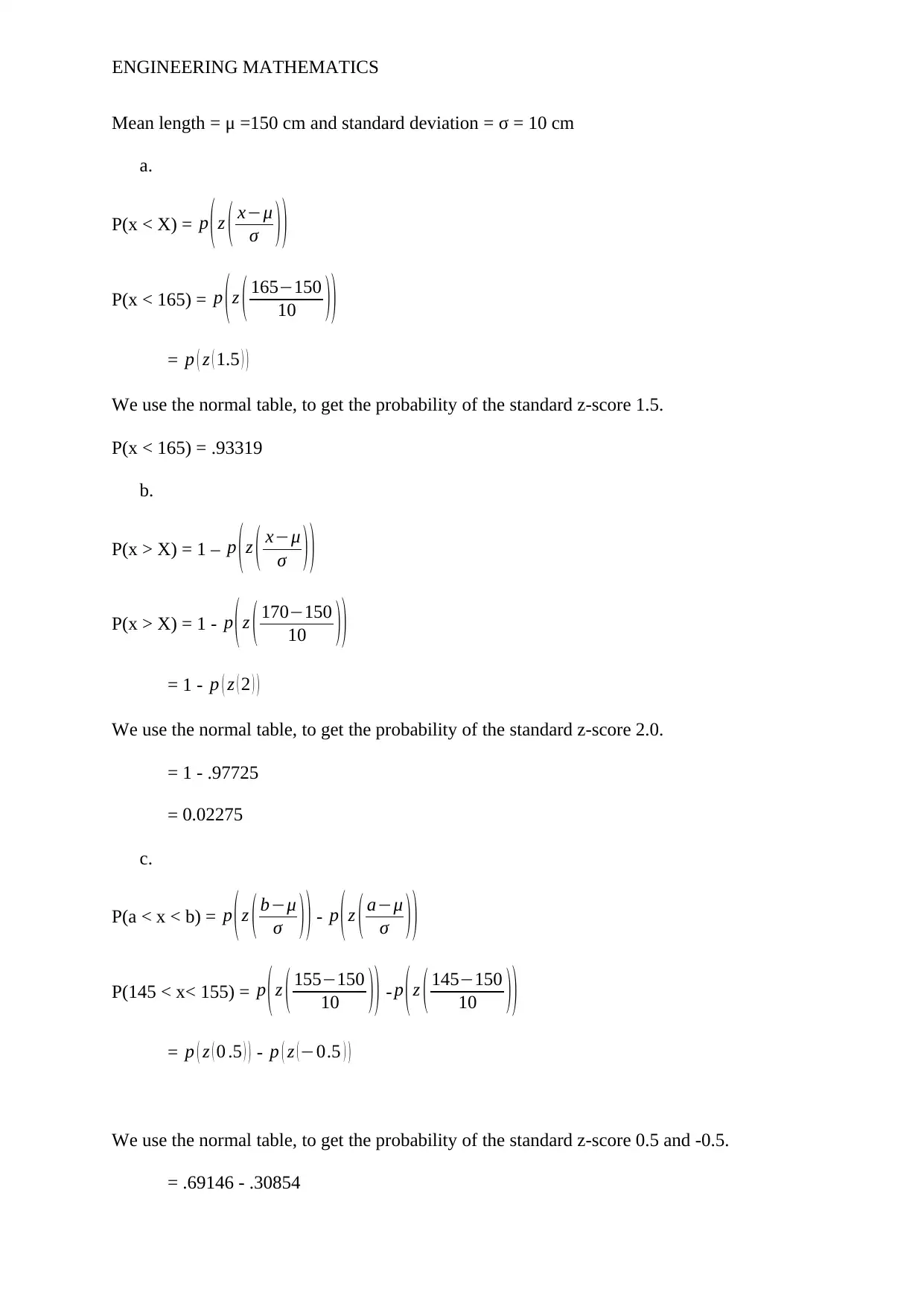
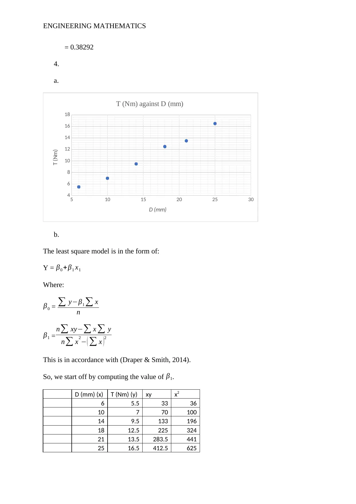
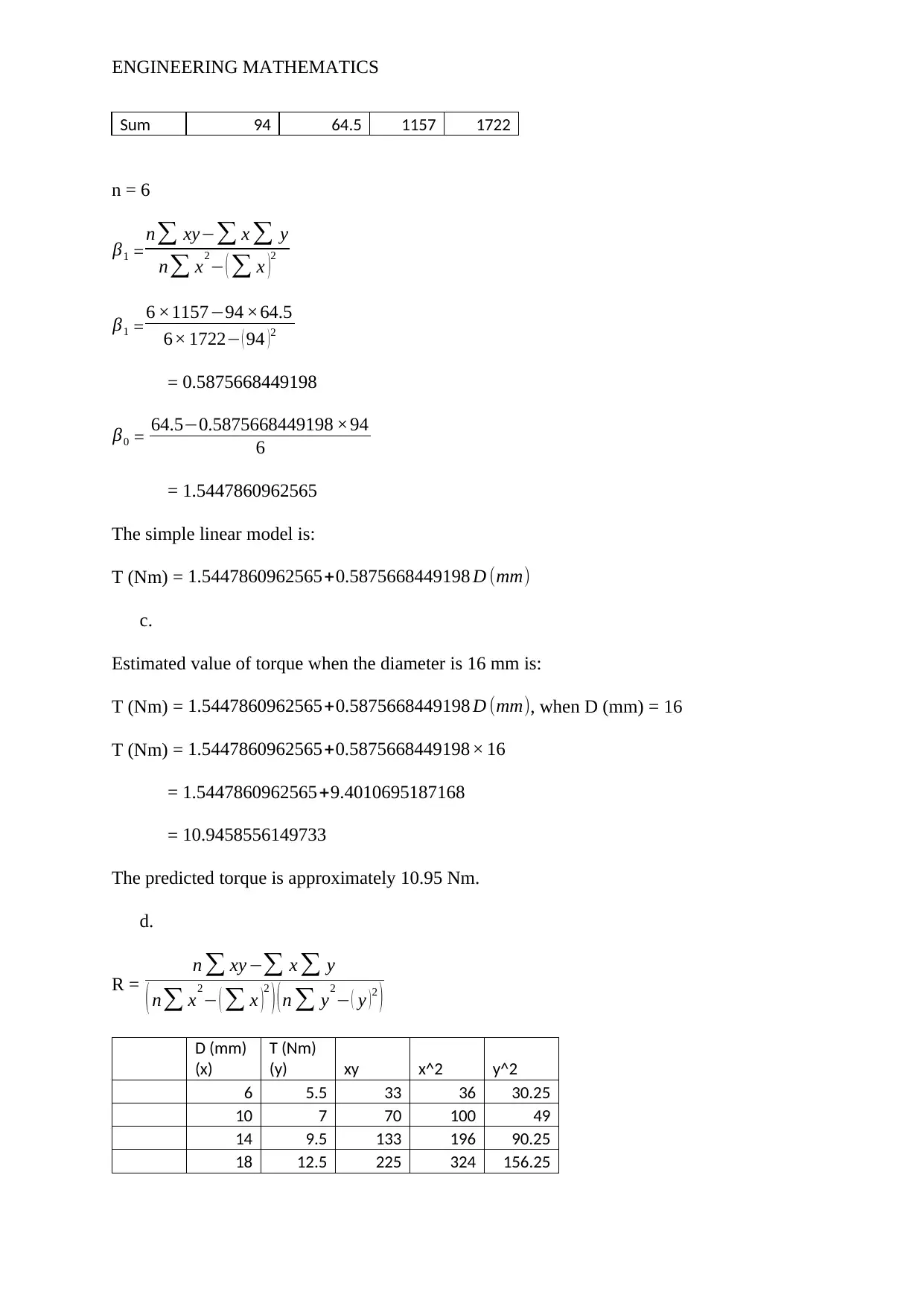
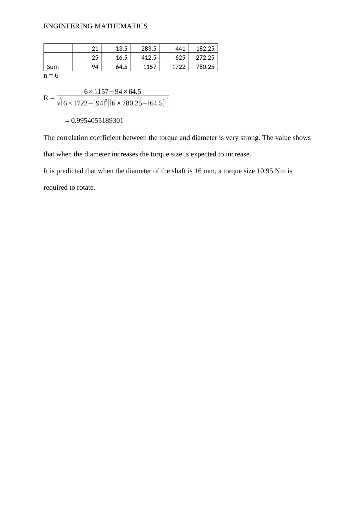
This assignment provides solutions to problems in engineering mathematics, focusing on statistics and probability. It includes calculations of the mean and standard deviation for grouped data, decision tree analysis for probability calculations, normal distribution problems, and linear regression analy...Read More

Running head: ENGINEERING MATHEMATICS
Engineering Mathematics
Name:
Institution:

ENGINEERING MATHEMATICS
1.
The mean of the grouped data is obtained using the formula:
Mean = ∑ fx
∑ f
Days lost Frequency (f) mid-point (x) fx
1–3 8 2 8×2 =
16
4–6 7 5 7×5 =
35
7–9 10 8 10×8 =
80
10-12 9 11 9×11 =
99
13-15 6 12 6×12 =
72
40 302
= 302
40
= 7.55
Standard deviation =
√ ∑ f ( x−x )2
∑ f
Days
lost
Frequenc
y (f) mid-point (x) ( x−x ) 2 f ( x−x ) 2
1–3 8 2 ( 2−7.55 )2 =
30.8025
8×30.8025 =
246.42
4–6 7 5
( 5−7.55 ) 2 =
6.5025
7×6.5025 =
45.5175
7–9 10 8
( 8−7.55 )2 =
0.2025
10×6.5025 =
2.025
10-12 9 11 ( 11−7.55 )2 =
11.9025
9×11.9025 =
107.123
13-15 6 12
( 12−7.55 )2 =
19.8025
6×19.8025 =
118.815
40 519.9
Std. dev = √ 5 1 9 . 9
40
= √ 12.9975

ENGINEERING MATHEMATICS
= 3.6052045711721
2.
a.
The decision tree is as illustrated below.
b.
i)
P (A and D) = p(A)×p(D)
= 0.60×0.02
= 0.012
ii)
This is obtained from either company A or company B
Probability of defective = p(defective from A) or p(defective from B)
= 0.60×0.02 + 0.40×0.01
= 0.012 + 0.004
= 0.016
iii)
P(D|A) = P (A and D)/P(D)
= 0.012/0.016
= 0.75
3.

ENGINEERING MATHEMATICS
Mean length = μ =150 cm and standard deviation = σ = 10 cm
a.
P(x < X) = p (z ( x−μ
σ ) )
P(x < 165) = p ( z ( 165−150
10 ))
= p ( z ( 1.5 ) )
We use the normal table, to get the probability of the standard z-score 1.5.
P(x < 165) = .93319
b.
P(x > X) = 1 – p (z ( x−μ
σ ) )
P(x > X) = 1 - p ( z ( 170−150
10 ))
= 1 - p ( z ( 2 ) )
We use the normal table, to get the probability of the standard z-score 2.0.
= 1 - .97725
= 0.02275
c.
P(a < x < b) = p (z ( b−μ
σ ) ) - p ( z ( a−μ
σ ) )
P(145 < x< 155) = p ( z ( 155−150
10 )) - p ( z ( 145−150
10 ))
= p ( z ( 0 .5 ) ) - p ( z (−0.5 ) )
We use the normal table, to get the probability of the standard z-score 0.5 and -0.5.
= .69146 - .30854

ENGINEERING MATHEMATICS
= 0.38292
4.
a.
5 10 15 20 25 30
4
6
8
10
12
14
16
18
T (Nm) against D (mm)
D (mm)
T (Nm)
b.
The least square model is in the form of:
Y = β0 +β1 x1
Where:
β0 = ∑ y−β1 ∑ x
n
β1 = n∑ xy−∑ x ∑ y
n∑ x2
− ( ∑ x )
2
This is in accordance with (Draper & Smith, 2014).
So, we start off by computing the value of β1.
D (mm) (x) T (Nm) (y) xy x2
6 5.5 33 36
10 7 70 100
14 9.5 133 196
18 12.5 225 324
21 13.5 283.5 441
25 16.5 412.5 625

ENGINEERING MATHEMATICS
Sum 94 64.5 1157 1722
n = 6
β1 = n∑ xy−∑ x ∑ y
n∑ x2
− ( ∑ x )
2
β1 = 6 ×1157−94 ×64.5
6× 1722− ( 94 ) 2
= 0.5875668449198
β0 = 64.5−0.5875668449198 ×94
6
= 1.5447860962565
The simple linear model is:
T (Nm) = 1.5447860962565+0.5875668449198 D (mm)
c.
Estimated value of torque when the diameter is 16 mm is:
T (Nm) = 1.5447860962565+0.5875668449198 D (mm), when D (mm) = 16
T (Nm) = 1.5447860962565+0.5875668449198× 16
= 1.5447860962565+9.4010695187168
= 10.9458556149733
The predicted torque is approximately 10.95 Nm.
d.
R =
n ∑ xy −∑ x ∑ y
( n∑ x2
− ( ∑ x )2
) ( n ∑ y2
− ( y )2 )
D (mm)
(x)
T (Nm)
(y) xy x^2 y^2
6 5.5 33 36 30.25
10 7 70 100 49
14 9.5 133 196 90.25
18 12.5 225 324 156.25

ENGINEERING MATHEMATICS
21 13.5 283.5 441 182.25
25 16.5 412.5 625 272.25
Sum 94 64.5 1157 1722 780.25
n = 6
R = 6× 1157−94 ×64.5
√ ( 6 ×1722− ( 94 )2 ) (6 × 780.25− ( 64.5 )2 )
= 0.9954055189301
The correlation coefficient between the torque and diameter is very strong. The value shows
that when the diameter increases the torque size is expected to increase.
It is predicted that when the diameter of the shaft is 16 mm, a torque size 10.95 Nm is
required to rotate.

ENGINEERING MATHEMATICS
References
Draper, N. R., & Smith, H. (2014). Applied regression analysis (Vol. 326). John Wiley &
Sons.