Probability and Statistics Assignment: Solutions and Analysis - 2020
VerifiedAdded on 2022/08/30
|14
|843
|13
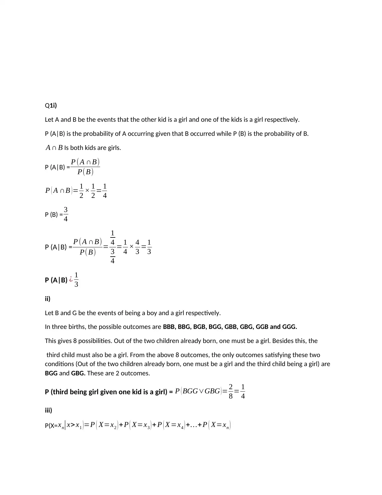
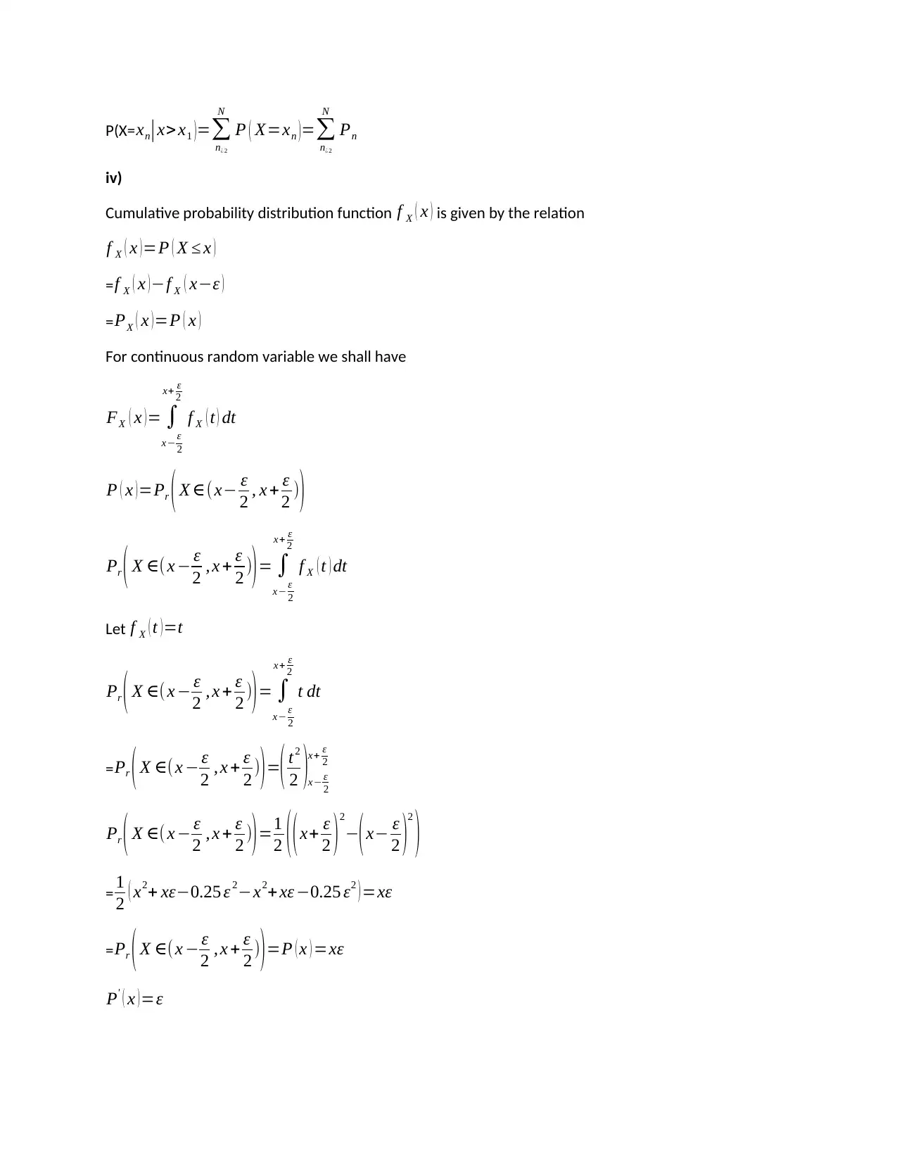
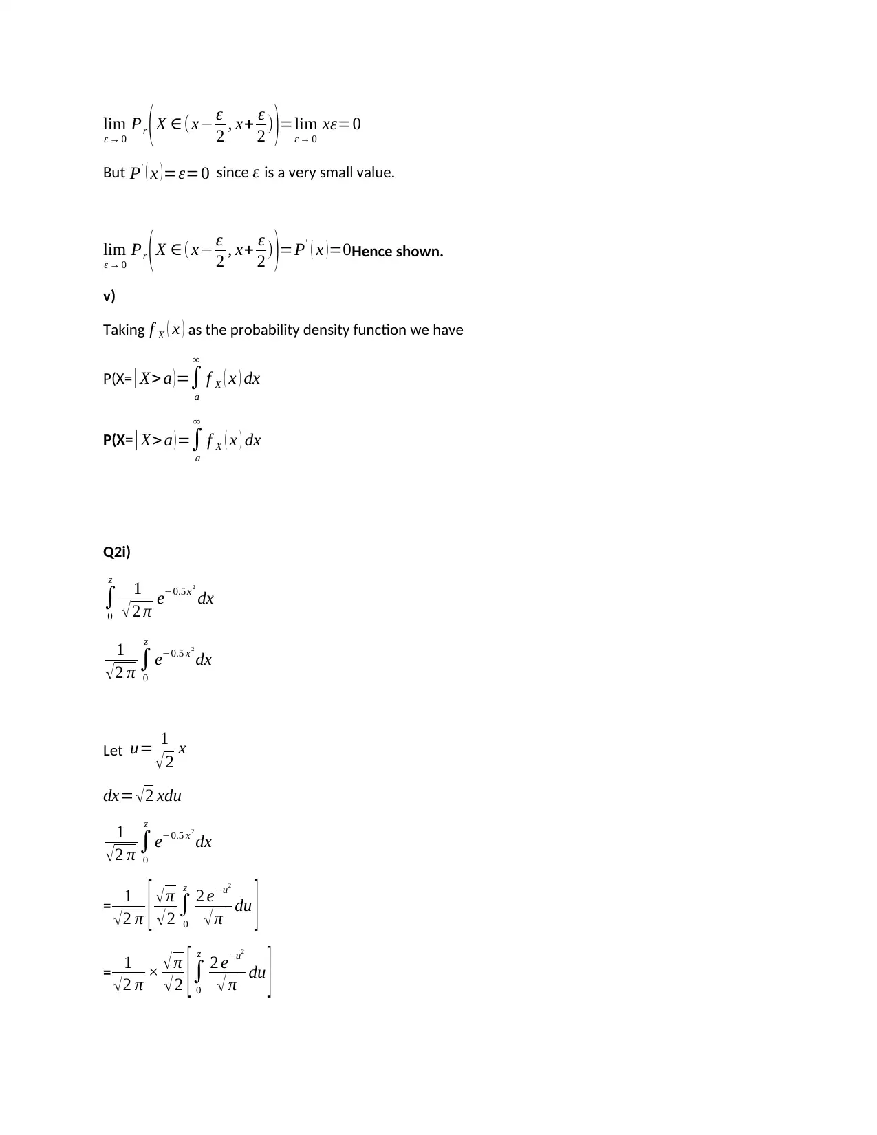
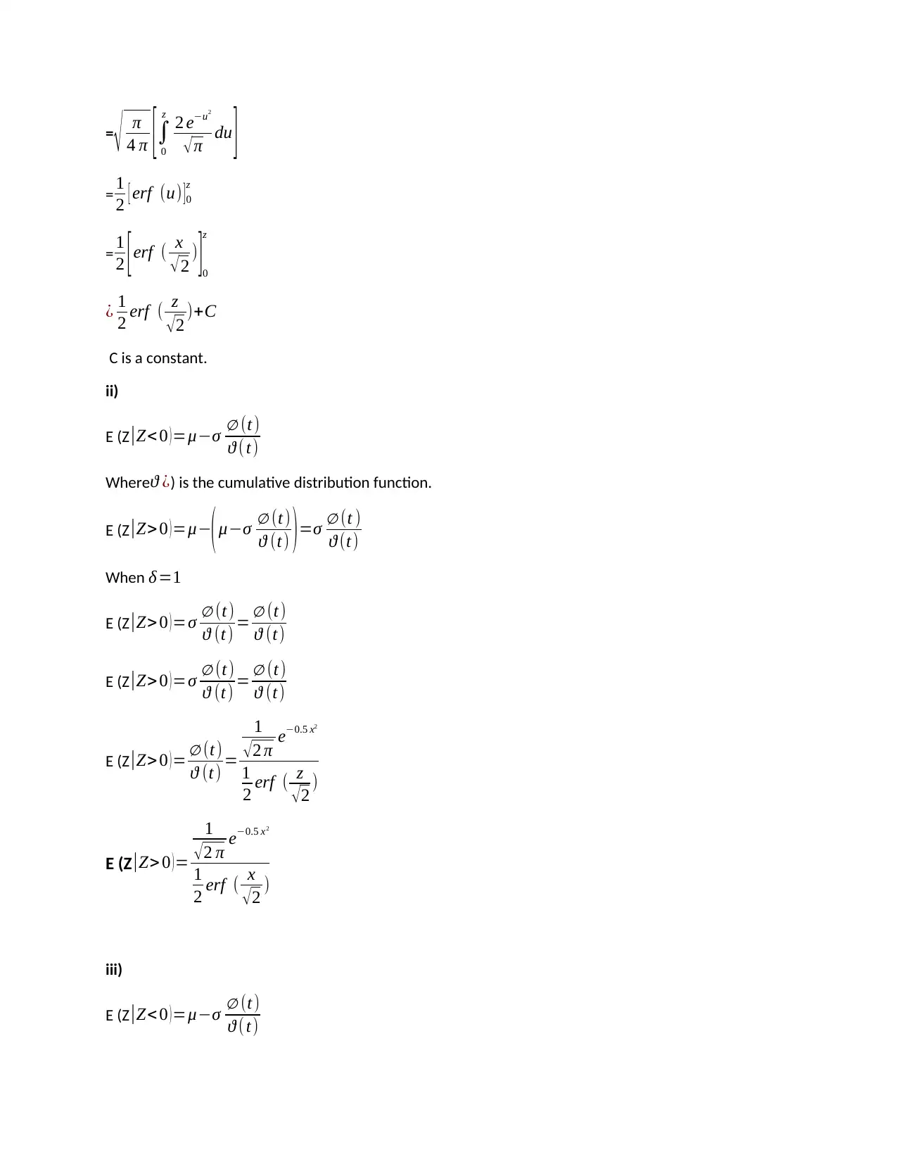
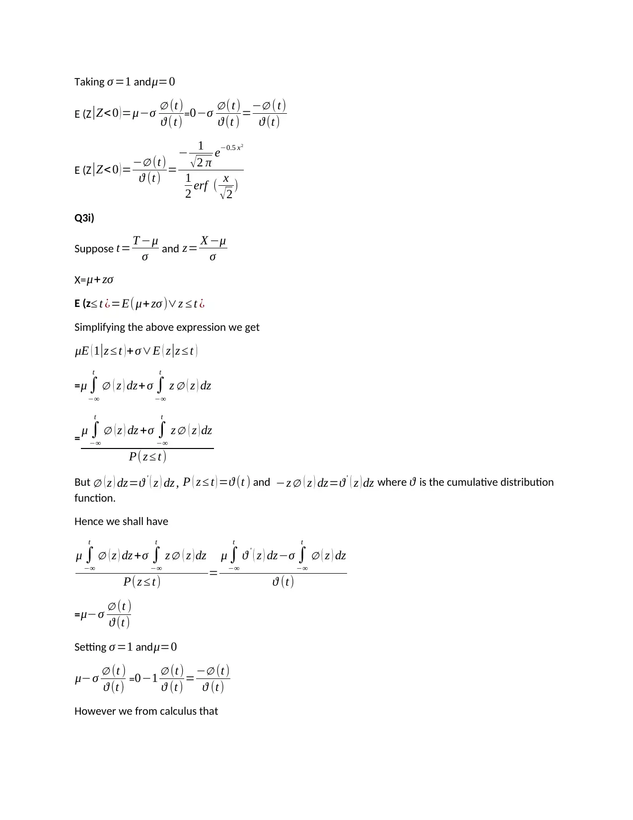
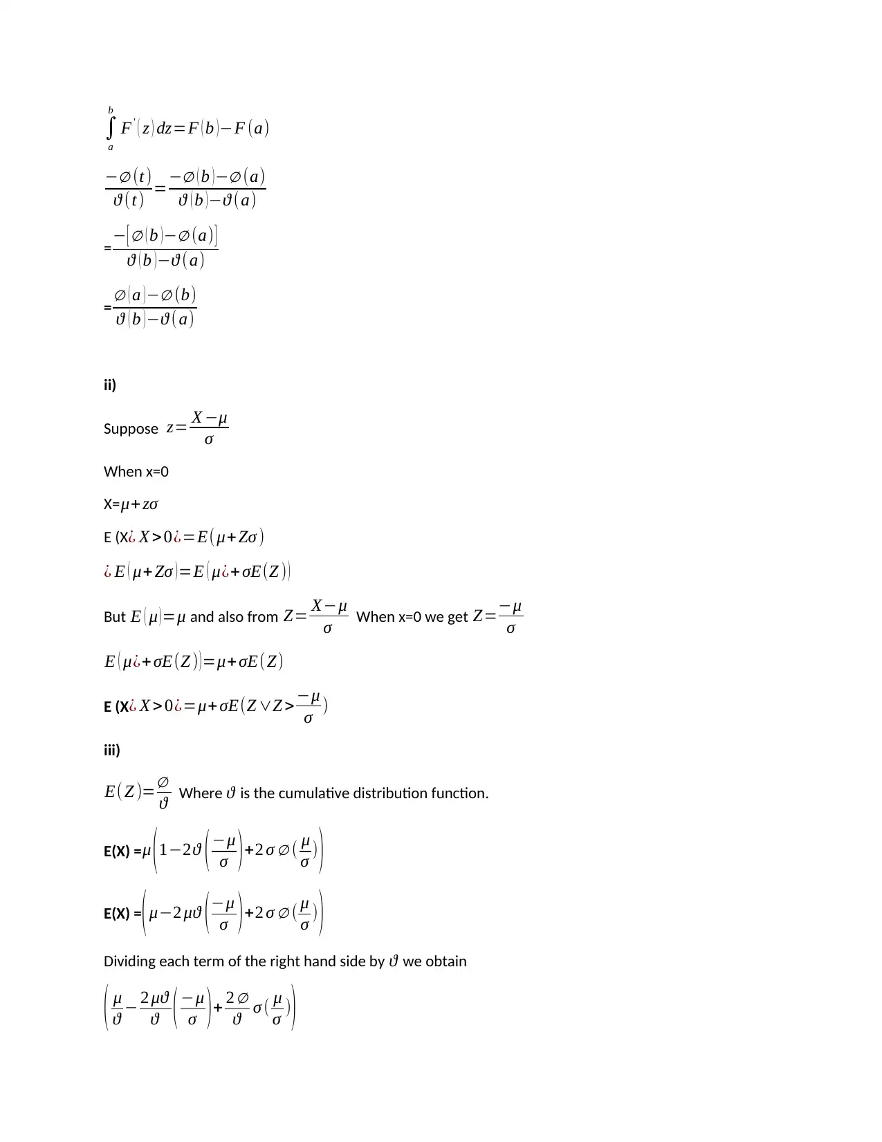
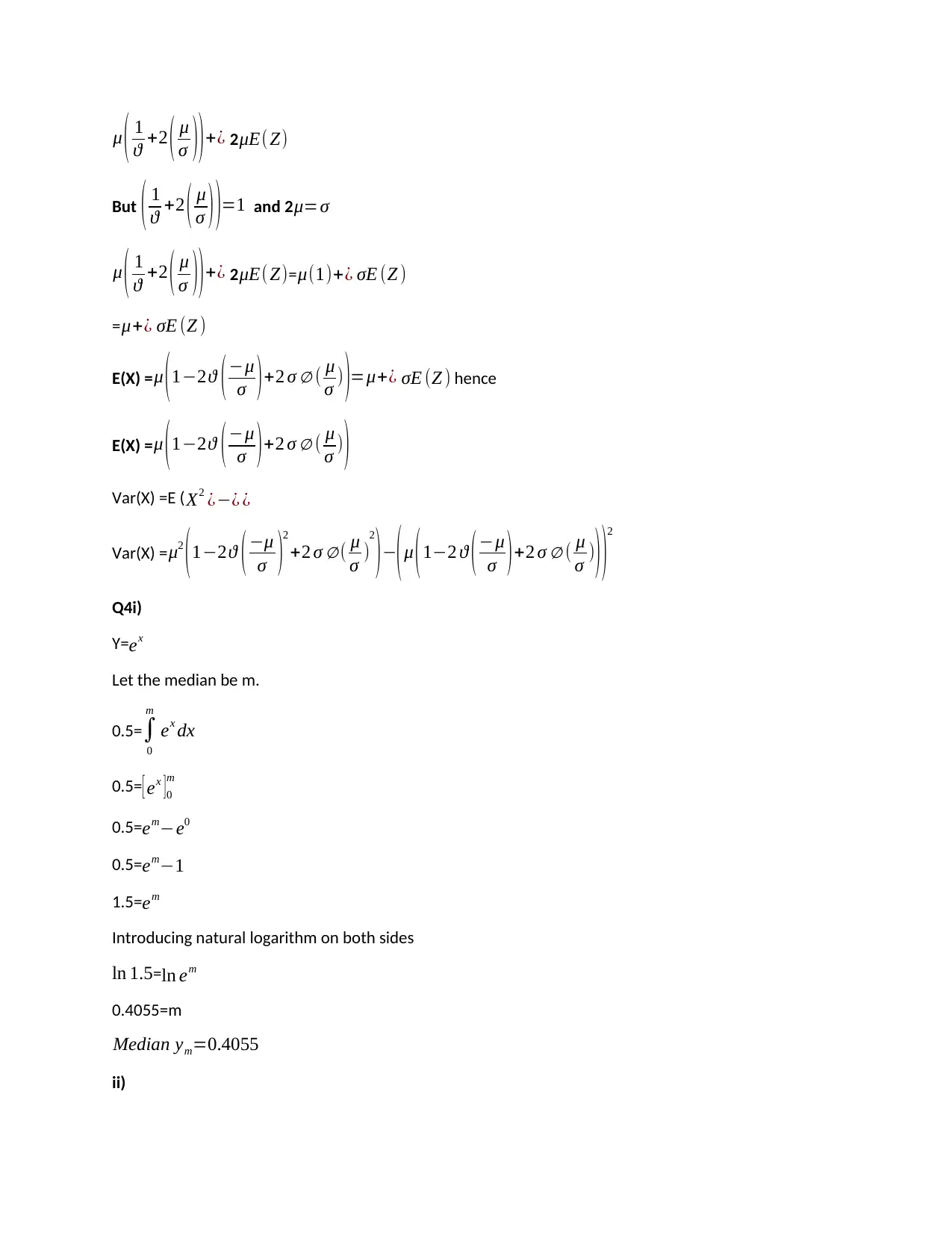
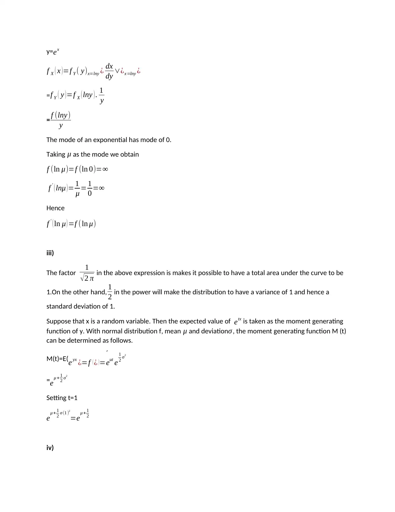
Homework Assignment
AI Summary
This document presents a comprehensive solution to a Mathematics assignment focusing on probability and statistics. The assignment covers a range of topics, including conditional probability, calculating probabilities in different scenarios (like the gender of children), and understanding cumulative probability distribution functions. It delves into expected values, variance, and moment-generating functions, demonstrating their application in solving statistical problems. Furthermore, the solution explores the diffusion equation, transition density, and long-run probabilities, providing a complete analysis of the concepts. The assignment is a valuable resource for students studying probability and statistics, offering detailed explanations and step-by-step solutions to enhance understanding and problem-solving skills.

1 out of 14
Related Documents


Your All-in-One AI-Powered Toolkit for Academic Success.
+13062052269
info@desklib.com
Available 24*7 on WhatsApp / Email
![[object Object]](/_next/static/media/star-bottom.7253800d.svg)
Copyright © 2020–2026 A2Z Services. All Rights Reserved. Developed and managed by ZUCOL.