Statistics Homework Project 3 - Statistical Analysis and Forecasting
VerifiedAdded on 2021/01/01
|33
|4662
|54
Homework Assignment
AI Summary
This homework project presents solutions to several statistical problems, including regression analysis and forecasting. The project analyzes data related to annual earnings, arsenic levels, gas turbine performance, and silicon wafer microchip failure times. It utilizes least squares regression to build predictive models and assesses the significance of variables. Additionally, the project explores time series forecasting techniques, such as moving averages, exponential smoothing, and Holt-Winters methods, to forecast the S&P index. The analysis includes interpreting coefficients, evaluating model fit (R-squared), and assessing the accuracy of forecasts. The document provides detailed calculations, interpretations, and conclusions for each exercise, offering a comprehensive understanding of the statistical concepts and techniques applied.

HOMEWORK PROJECT 3 1
Homework Project3
Homework Project3
Paraphrase This Document
Need a fresh take? Get an instant paraphrase of this document with our AI Paraphraser

Table of Contents
1. Title page ………………………………………………………………….…….1
2. Table of contents ………………………………………………………….……..2
3. Honesty statement……………………………………………………….……….3
4. Exercise
4.6..........................................................................................................................3
5. Exercise
4.12........................................................................................................................4
6. Exercise
4.24........................................................................................................................5
7. Exercise
4.32........................................................................................................................6
8. Exercise
4.40........................................................................................................................7
9. Exercise
6.6..........................................................................................................................8
10. Exercise
10.6........................................................................................................................9
11. Exercise
10.2......................................................................................................................12
12. Exercise
10.3......................................................................................................................13
13. Appendices..........................................................................................................14

Honesty Statement
I, Betsy Sophia Reed, promise that I did not reference or use any previous solutions or statistics
in this submission. I promise that all exercises are my original work and that no other individual,
including a tutor, performed these statistics.
I, Betsy Sophia Reed, promise that I did not reference or use any previous solutions or statistics
in this submission. I promise that all exercises are my original work and that no other individual,
including a tutor, performed these statistics.
⊘ This is a preview!⊘
Do you want full access?
Subscribe today to unlock all pages.
Trusted by 1+ million students worldwide
Exercise 4.6 is about least square prediction of annual earnings based on age and working hours.
Earnings of Mexican street vendors
Detailed interviews were conducted with over 1,000 street vendors in the city of Puebla, Mexico,
in order to study the factors influencing vendors’ incomes
(4.6.a)
The first order model for mean of annual earning as a function of age (x1) and hours worked (x2)
would be:
E(y) = α + β1 X1 + β2 X2 + e
(4.6.b)Least square prediction equation:
Y = -20.352 + 13.350 X1 + 243.714 X2+ e
(4.6.c)
The least square prediction equation has two β in the equation, which is β1 and β2. β1 is the
coefficient of age, which values 13.350. It means that if there is one year addition to the age, then
the annual earnings will increase to 13.350. In the other hand, β2 is the coefficient of hours
worked which values 243.714. It means that if there is one hour addition to the working hours
then the annual earnings will increase 243.714.
(4.6.d)
The global utility of the model can be seen from F-test probability. With significance level of
1%, age and hours worked are significantly influencing the annual earnings (p < 0.01).
(4.6.e)
Paraphrase This Document
Need a fresh take? Get an instant paraphrase of this document with our AI Paraphraser
58.2% of annual earnings prediction can be explained by age and hours worked (R2= 0.582).
41.8% of annual earnings are explained by other factors which is not included in the model.
(4.6.f)
The standard error of estimate is 547.737, which means that the measurement of variability in
estimation of annual earnings is around 547.737.
(4.6.g)
Age (x1) have t-test probability of 0.107, which is larger than the significance level (α = 0.01).
Therefore, age is not significantly affecting annual earnings.
(4.6.h)
The confidence interval of β2 is from 105.334 to 382.095, which means that the additional annual
earnings if 1 hour of working hours is added would be around 105.334 to 382.095.
Exercise 4.12 is about modelling arsenic level as a function of latitude, longitude, and depth. We
use least squares model to predict the arsenic level.
(4.12.a)
E(y) = α + β1 X1 + β2 X2 + β3 X3 e
Where y = arsenic level, X1= latitude, X2= longitude, X3 = depth.
(4.12.b)
Y = -86867.917 – 2218.757 X1 + 1542.163 X2 – 0.350 X3 + e
(4.12.c)
There are three beta coefficient in the model. The β1 values -2218.757 which means that if
latitude rises 1, then the arsenic level will decrease 2218.757. If longitude is added by 1, then the
arsenic level will increase 1542.163. However, if depth is added by 1, then the arsenic level will
decrease 0.350.
(4.13.d)
The estimate value of arsenic level will deviate up to 10671.180 (s = 10671.180).
(4.13.e)
12.8% of variations in arsenic level value can be explained by latitude, longitude, and depth (R2
= 0.128). However, if we adjust it, only 12% of variations in arsenic level value can be explained
by latitude, longitude, and depth (R2a = 0.120).
(4.13.f)
The model which is arsenic level building by latitude, longitude, and depth is statistically
significant and useful (F = 15.799, p-value = 0.000).
(4.13.g)
I will use three predictors, which is latitude, longitude, and depth. However, I will also add
another variable that might explain the arsenic level better. I will not delete those 3 variables
because those variables are statistically significant whether by t-test of F-test, but the R2 still
need to be higher.
Exercise 4.24 – Cooling Method of Gas Turbine
The Journal for Engineering for Gas Turbines and Power study of a high pressure inlet fogging
method for a gas turbine engine
(4.24.a)
The prediction interval for y (12157.9, 13107.1) means that the predicted heat rate is from
12157.9 to 13107.1 with 95% of confidence level
(4.24.b)
The prediction interval for E(y) (11599.6, 13665.5) means that the expected heat rate is from
11599.6 to 13665.5 with 95% of confidence level.
(4.24.c)
⊘ This is a preview!⊘
Do you want full access?
Subscribe today to unlock all pages.
Trusted by 1+ million students worldwide
The prediction interval for y is narrower than interval for E(y) because the prediction relies on
the model. However, the E(y) only depends on the Y value, so it’s broader than prediction
interval for y.
Exercise 4.32 Cooling Method for Gas Turbines is about interaction model in predicting
heat rate based on inlet & exhaust temperature and air flow
(4.32.a)
Regression Equation
E (Y) = β0 + β1X1 + β2X2 + β3X3 + β4X4 + β5X5
Dependent variables: Heart rate
Independent variables: Functions of speed, inlet temperature, exhaust temperature, cycle
pressure ratio and air flow rate
(4.32.b)
Y = 13944.728 – 15.138 X2 + 28.843 X3 – 0.689 X5 + 0.023 X2*X5 – 0.054 X3*X5 + e
X2 = inlet temperature, X3 = exhaust temperature, X5 = air flow
(4.32.c)
Inlet temperature and air flow interaction are presented by β4. It has p-value of 0.000 (p < 0.05),
which means that the interaction of inlet temperature and air flow interaction is significantly
affecting the heat rate.
(4.32.d)
Exhaust temperature and air flow interaction are presented by β5. It has p-value of 0.000 (p <
0.05), which means that the interaction of exhaust temperature and air flow interaction is
significantly affecting the heat rate.
(4.32.e)
Paraphrase This Document
Need a fresh take? Get an instant paraphrase of this document with our AI Paraphraser
The interaction of inlet temperature and air flow is significantly affecting heat rate, which means
that inlet temperature depends on air flow rate. However, exhaust temperature and air flow
interaction is also significant, which indicates that exhaust temperature also depends on air flow
rate.
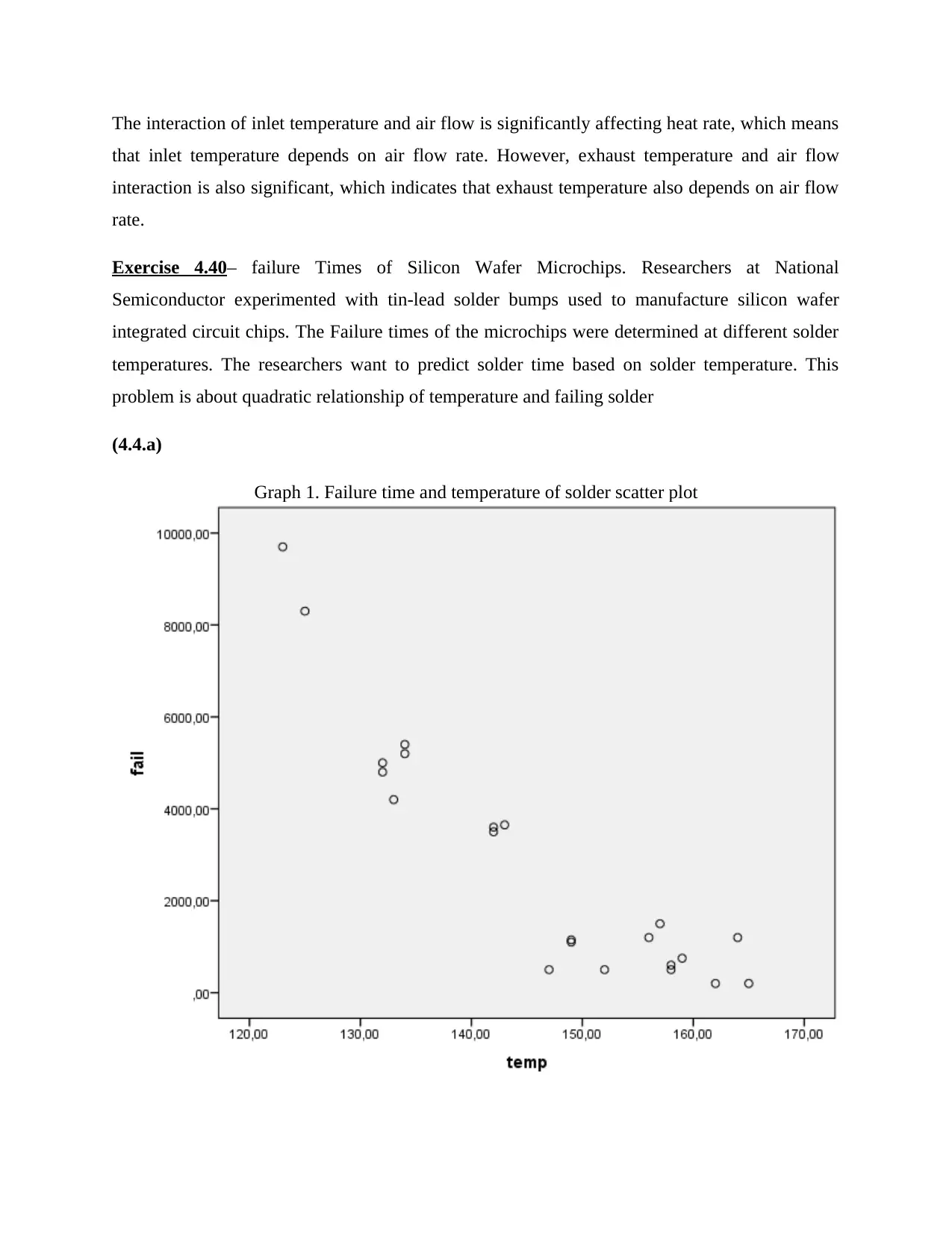
Exercise 4.40– failure Times of Silicon Wafer Microchips. Researchers at National
Semiconductor experimented with tin-lead solder bumps used to manufacture silicon wafer
integrated circuit chips. The Failure times of the microchips were determined at different solder
temperatures. The researchers want to predict solder time based on solder temperature. This
problem is about quadratic relationship of temperature and failing solder
(4.4.a)
Graph 1. Failure time and temperature of solder scatter plot
that inlet temperature depends on air flow rate. However, exhaust temperature and air flow
interaction is also significant, which indicates that exhaust temperature also depends on air flow
rate.
Exercise 4.40– failure Times of Silicon Wafer Microchips. Researchers at National
Semiconductor experimented with tin-lead solder bumps used to manufacture silicon wafer
integrated circuit chips. The Failure times of the microchips were determined at different solder
temperatures. The researchers want to predict solder time based on solder temperature. This
problem is about quadratic relationship of temperature and failing solder
(4.4.a)
Graph 1. Failure time and temperature of solder scatter plot
It’s shown in the graph that both variables might have quadratic relationship.
(4.40.b)
E(y) = 154242.914 – 1908.85 X + 5.929 X2
(4.40.c)
H0: β2 = 0
H1: β2 > 0
Based on the t-test probability, the coefficient β2 is significant (p < 0.05), which means that there
is upward curvature in the model.
Exercise 6.6 Clerical Staff Work Hours
This exercise is about selecting best model for predicting clerical’s staff working hours. In any
production process in which one or more workers are engaged in a variety of tasks, the total time
spent in production varies as a function of the size of the work pool and the level of output of the
various activities.
(6.6.a)
The final model selected by stepwise method:
Y = α + β1 X2 + β2 X4 + β3 X5 + e
(6.6.b)
Y = 77.726 + 0.136 X2 – 0.035 X4 + 0.058 X5
The coefficient of number of money orders and gift certificate sold (X2) values 0.136. It means
that if there is one addition of money orders and gift certificate sold, then the clerical’s staff
working hours will decrease 0.136 hour.
The coefficient of number of change order transaction processed (X4) values -0.035. It means
that if there is one addition in change order transaction, then the clerical’s staff working hours
will decrease 0.035 hour.
⊘ This is a preview!⊘
Do you want full access?
Subscribe today to unlock all pages.
Trusted by 1+ million students worldwide
The coefficient of number of checks cashed (X5) values 0.058. It means that if there is one
addition in checks cashed number, then the clerical’s staff working hours will increase 0.058
hour.
(6.6.c)
The inferences from stepwise model are affected by how many variables are actually building the
model. It may abolish important findings just because the inferences are not significant.
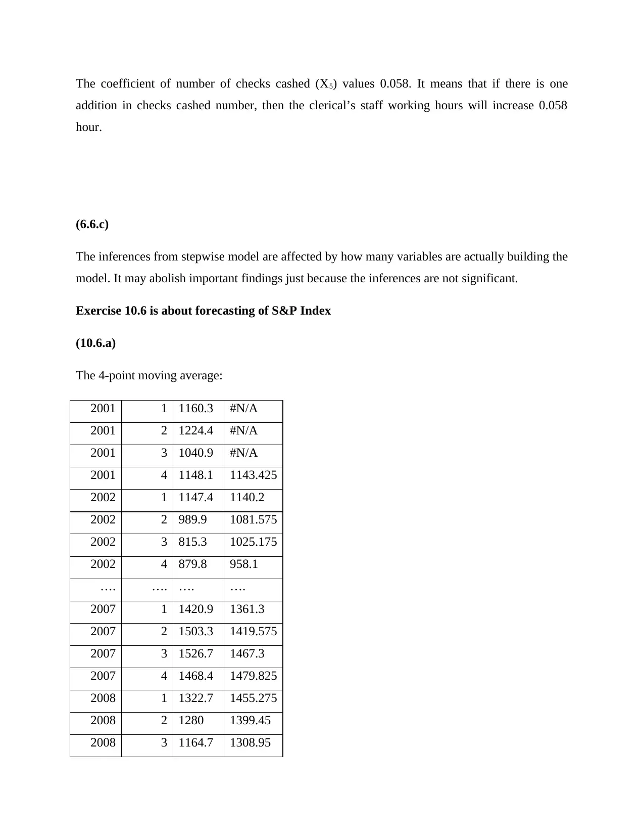
Exercise 10.6 is about forecasting of S&P Index
(10.6.a)
The 4-point moving average:
2001 1 1160.3 #N/A
2001 2 1224.4 #N/A
2001 3 1040.9 #N/A
2001 4 1148.1 1143.425
2002 1 1147.4 1140.2
2002 2 989.9 1081.575
2002 3 815.3 1025.175
2002 4 879.8 958.1
…. …. …. ….
2007 1 1420.9 1361.3
2007 2 1503.3 1419.575
2007 3 1526.7 1467.3
2007 4 1468.4 1479.825
2008 1 1322.7 1455.275
2008 2 1280 1399.45
2008 3 1164.7 1308.95
addition in checks cashed number, then the clerical’s staff working hours will increase 0.058
hour.
(6.6.c)
The inferences from stepwise model are affected by how many variables are actually building the
model. It may abolish important findings just because the inferences are not significant.
Exercise 10.6 is about forecasting of S&P Index
(10.6.a)
The 4-point moving average:
2001 1 1160.3 #N/A
2001 2 1224.4 #N/A
2001 3 1040.9 #N/A
2001 4 1148.1 1143.425
2002 1 1147.4 1140.2
2002 2 989.9 1081.575
2002 3 815.3 1025.175
2002 4 879.8 958.1
…. …. …. ….
2007 1 1420.9 1361.3
2007 2 1503.3 1419.575
2007 3 1526.7 1467.3
2007 4 1468.4 1479.825
2008 1 1322.7 1455.275
2008 2 1280 1399.45
2008 3 1164.7 1308.95
Paraphrase This Document
Need a fresh take? Get an instant paraphrase of this document with our AI Paraphraser
2008 4 903.3 1167.675
Table 1. 4-point moving average
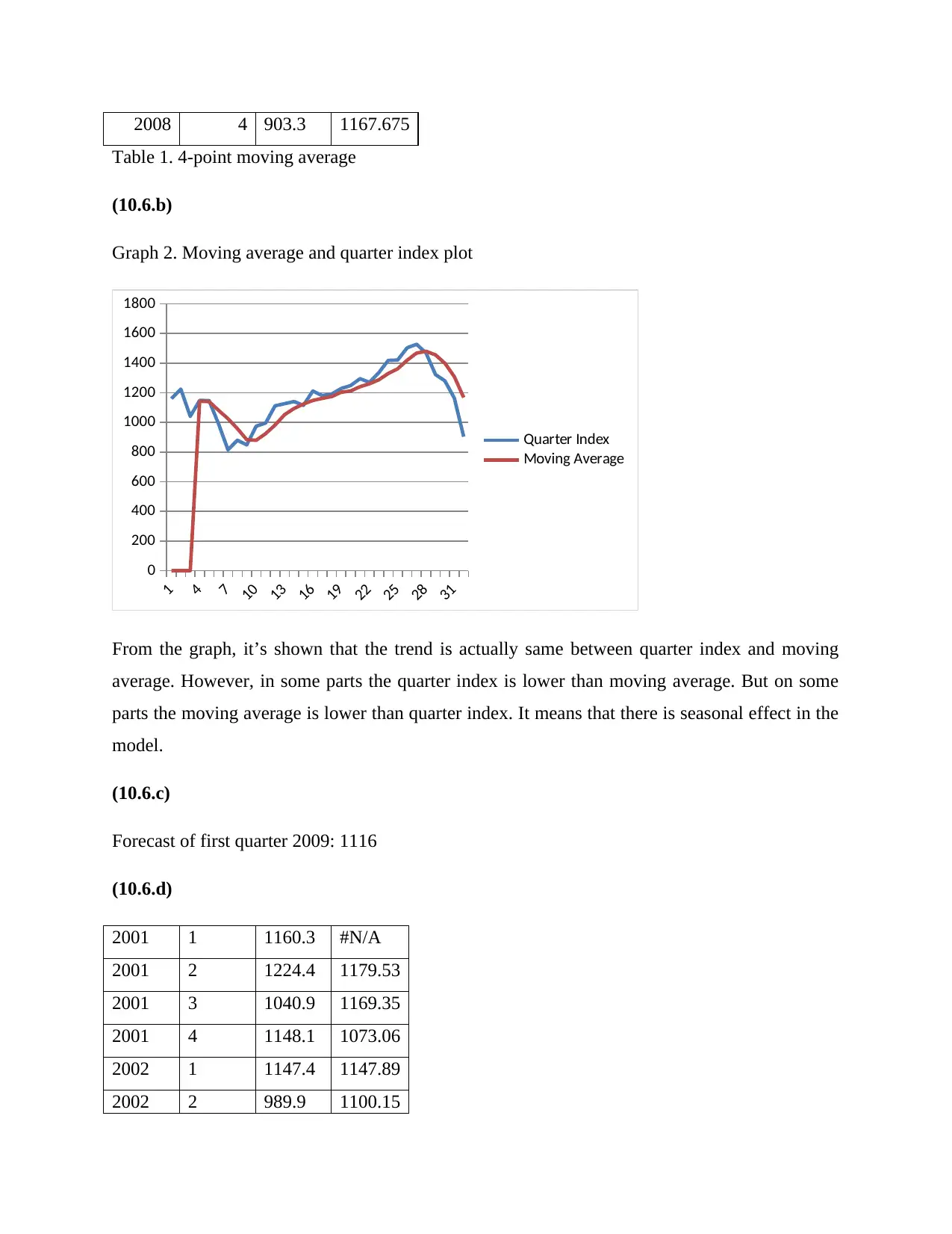
(10.6.b)
Graph 2. Moving average and quarter index plot
1
4
7
10
13
16
19
22
25
28
31
0
200
400
600
800
1000
1200
1400
1600
1800
Quarter Index
Moving Average
From the graph, it’s shown that the trend is actually same between quarter index and moving
average. However, in some parts the quarter index is lower than moving average. But on some
parts the moving average is lower than quarter index. It means that there is seasonal effect in the
model.
(10.6.c)
Forecast of first quarter 2009: 1116
(10.6.d)
2001 1 1160.3 #N/A
2001 2 1224.4 1179.53
2001 3 1040.9 1169.35
2001 4 1148.1 1073.06
2002 1 1147.4 1147.89
2002 2 989.9 1100.15
Table 1. 4-point moving average
(10.6.b)
Graph 2. Moving average and quarter index plot
1
4
7
10
13
16
19
22
25
28
31
0
200
400
600
800
1000
1200
1400
1600
1800
Quarter Index
Moving Average
From the graph, it’s shown that the trend is actually same between quarter index and moving
average. However, in some parts the quarter index is lower than moving average. But on some
parts the moving average is lower than quarter index. It means that there is seasonal effect in the
model.
(10.6.c)
Forecast of first quarter 2009: 1116
(10.6.d)
2001 1 1160.3 #N/A
2001 2 1224.4 1179.53
2001 3 1040.9 1169.35
2001 4 1148.1 1073.06
2002 1 1147.4 1147.89
2002 2 989.9 1100.15
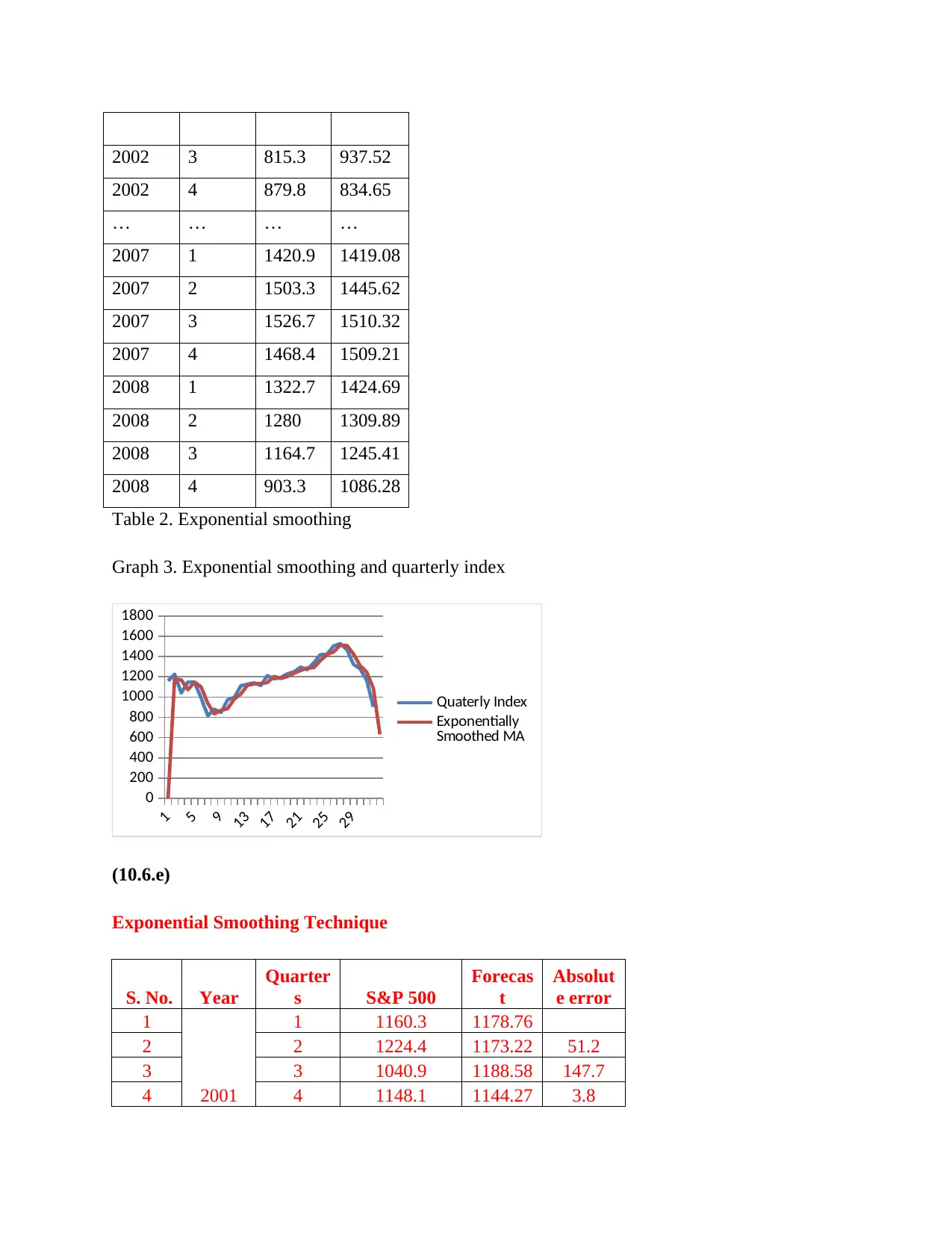
2002 3 815.3 937.52
2002 4 879.8 834.65
… … … …
2007 1 1420.9 1419.08
2007 2 1503.3 1445.62
2007 3 1526.7 1510.32
2007 4 1468.4 1509.21
2008 1 1322.7 1424.69
2008 2 1280 1309.89
2008 3 1164.7 1245.41
2008 4 903.3 1086.28
Table 2. Exponential smoothing
Graph 3. Exponential smoothing and quarterly index
1
5
9
13
17
21
25
29
0
200
400
600
800
1000
1200
1400
1600
1800
Quaterly Index
Exponentially
Smoothed MA
(10.6.e)
Exponential Smoothing Technique
S. No. Year
Quarter
s S&P 500
Forecas
t
Absolut
e error
1
2001
1 1160.3 1178.76
2 2 1224.4 1173.22 51.2
3 3 1040.9 1188.58 147.7
4 4 1148.1 1144.27 3.8
⊘ This is a preview!⊘
Do you want full access?
Subscribe today to unlock all pages.
Trusted by 1+ million students worldwide
1 out of 33

Your All-in-One AI-Powered Toolkit for Academic Success.
+13062052269
info@desklib.com
Available 24*7 on WhatsApp / Email
![[object Object]](/_next/static/media/star-bottom.7253800d.svg)
Unlock your academic potential
Copyright © 2020–2026 A2Z Services. All Rights Reserved. Developed and managed by ZUCOL.