HI6007 Statistics Assignment: Analyzing Business Data and Regression

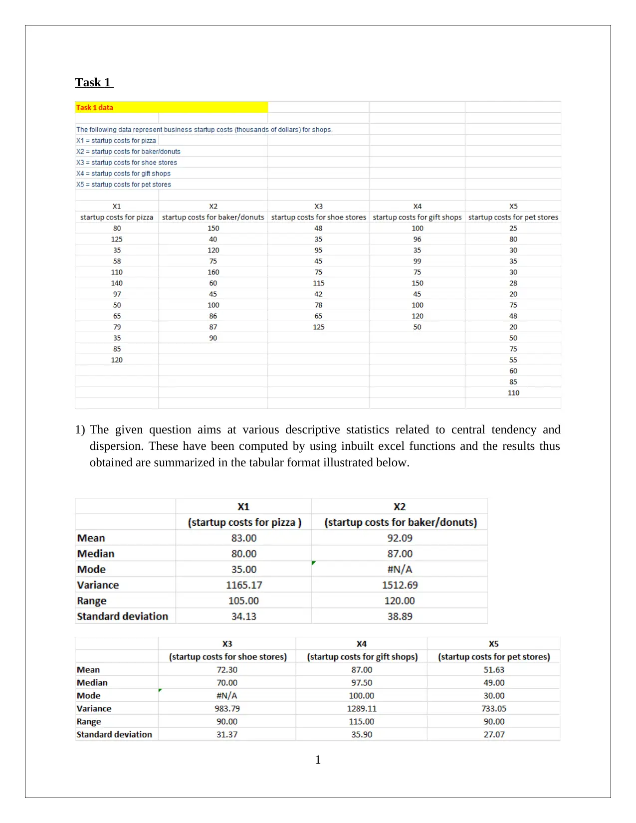
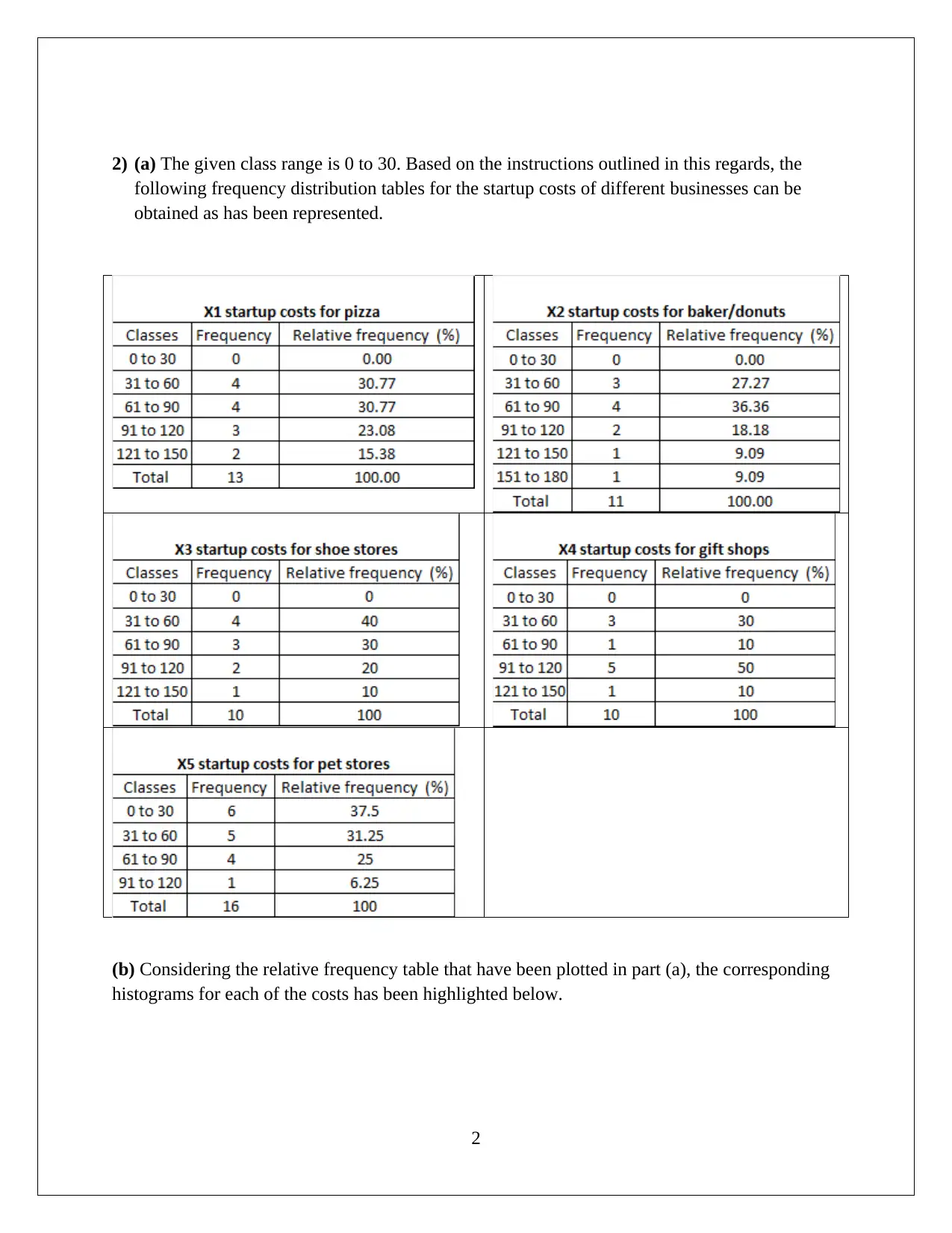
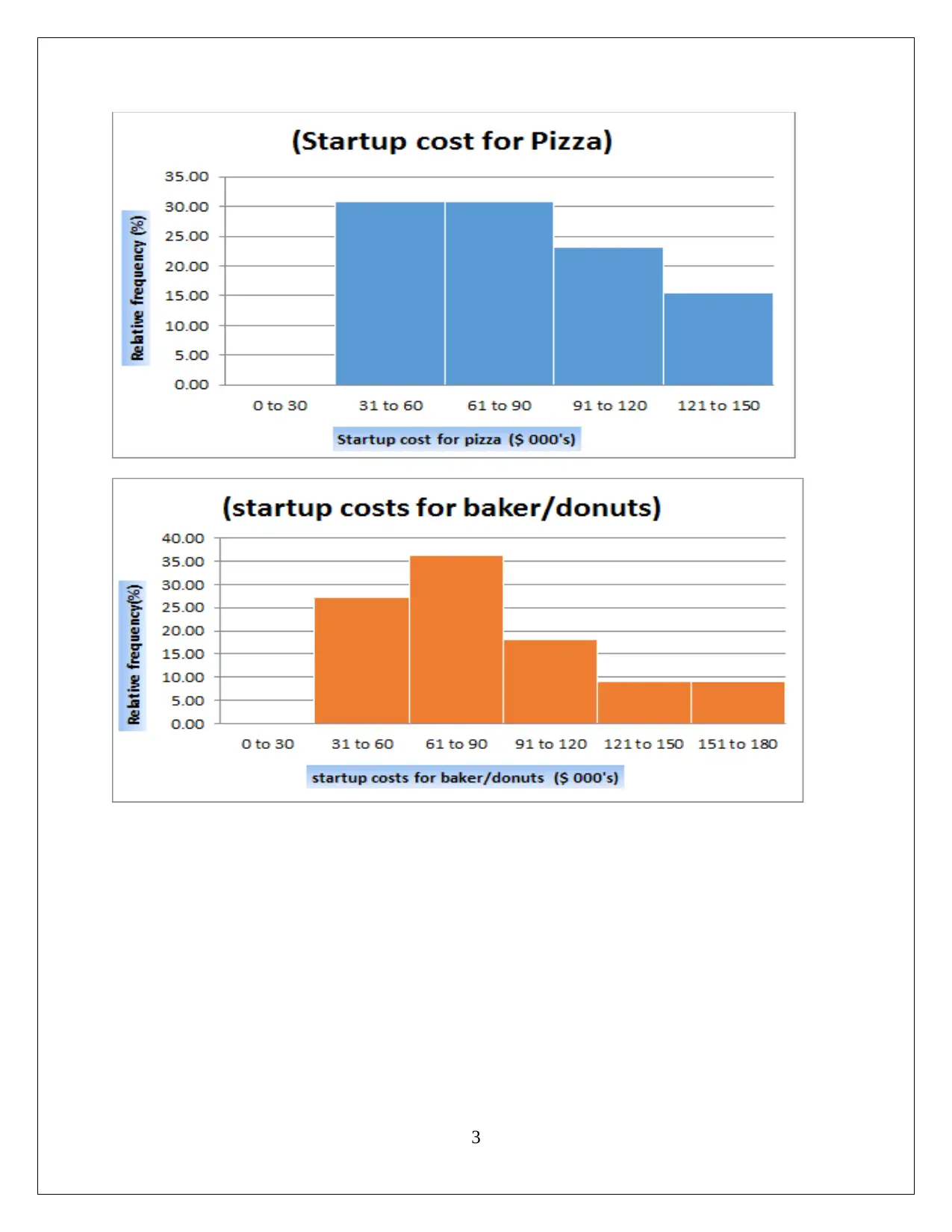
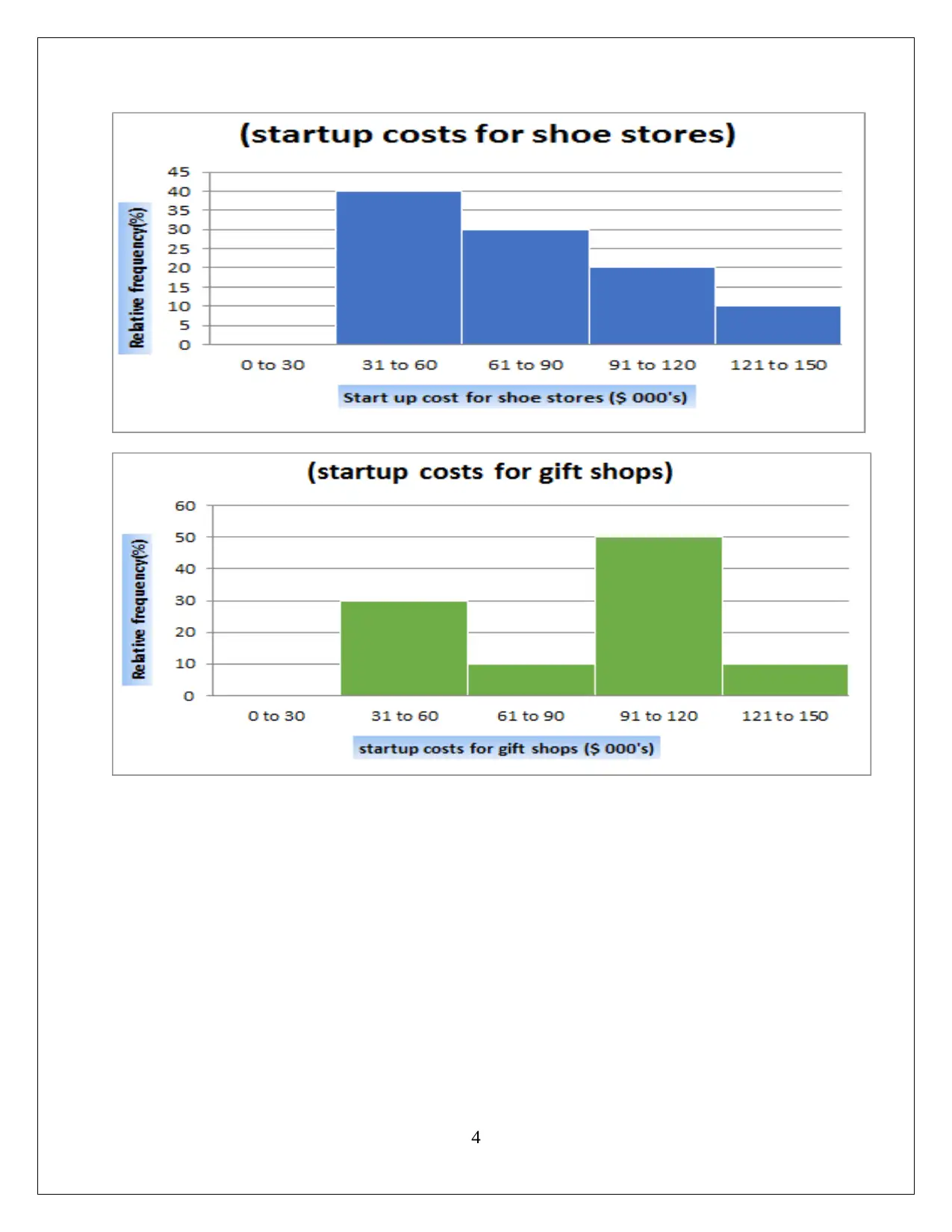
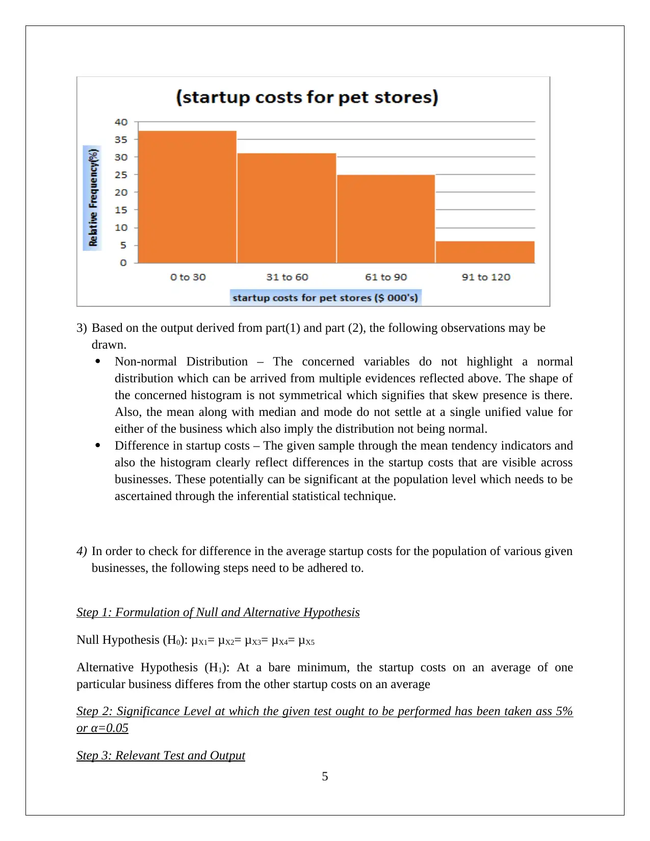
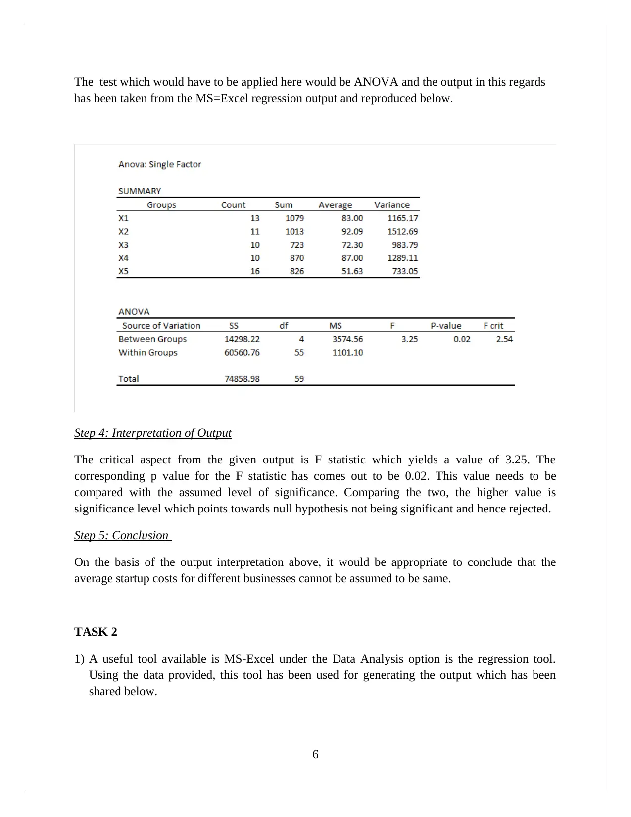
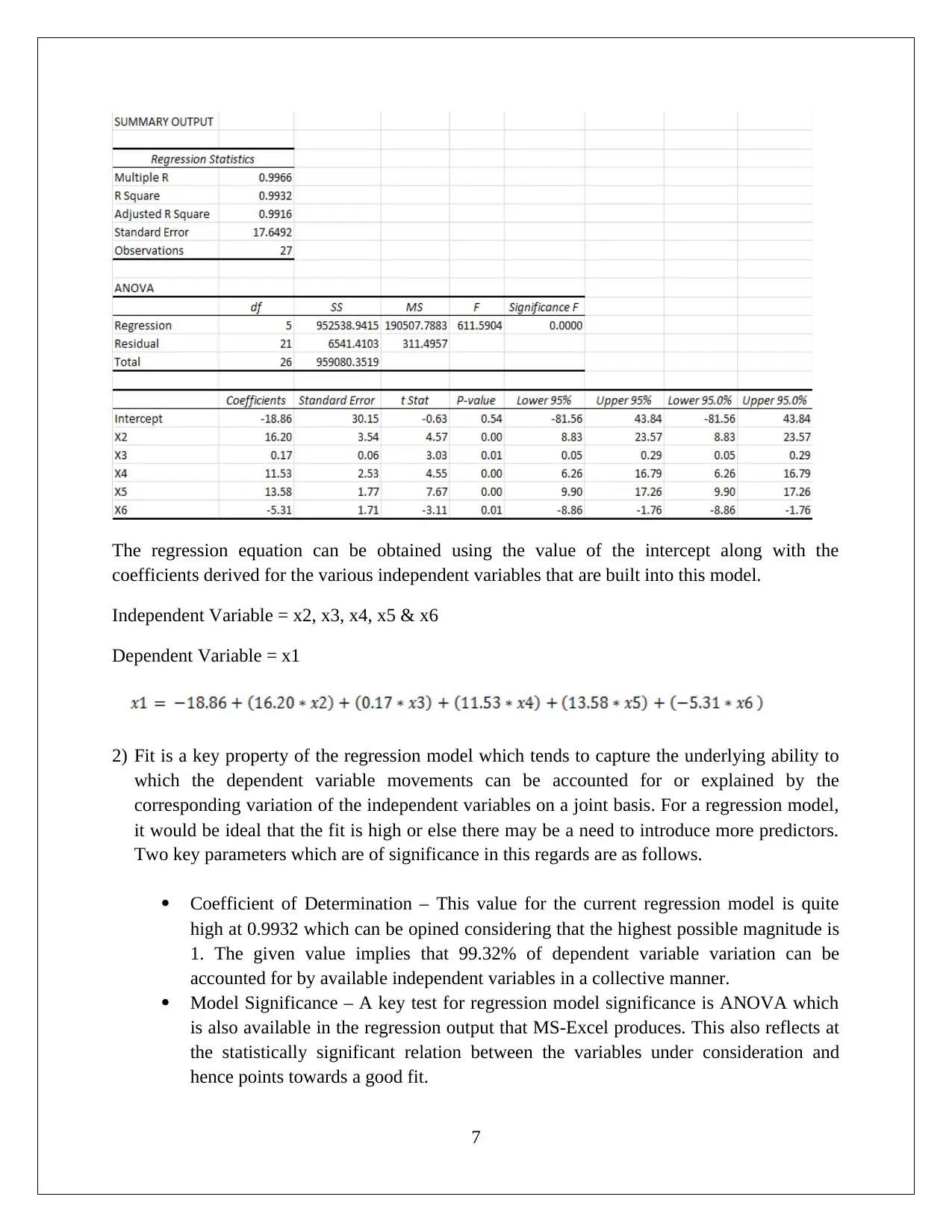
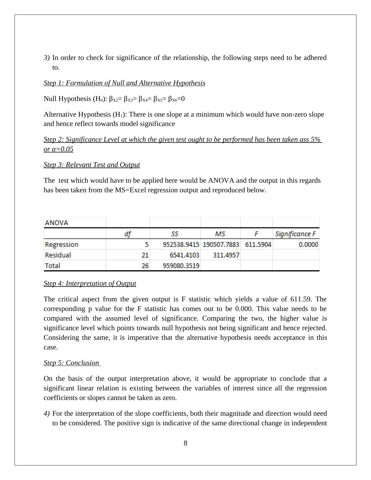
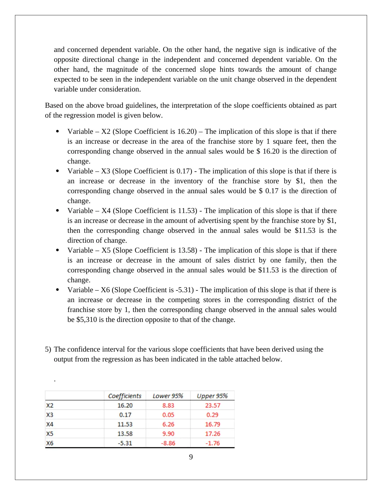
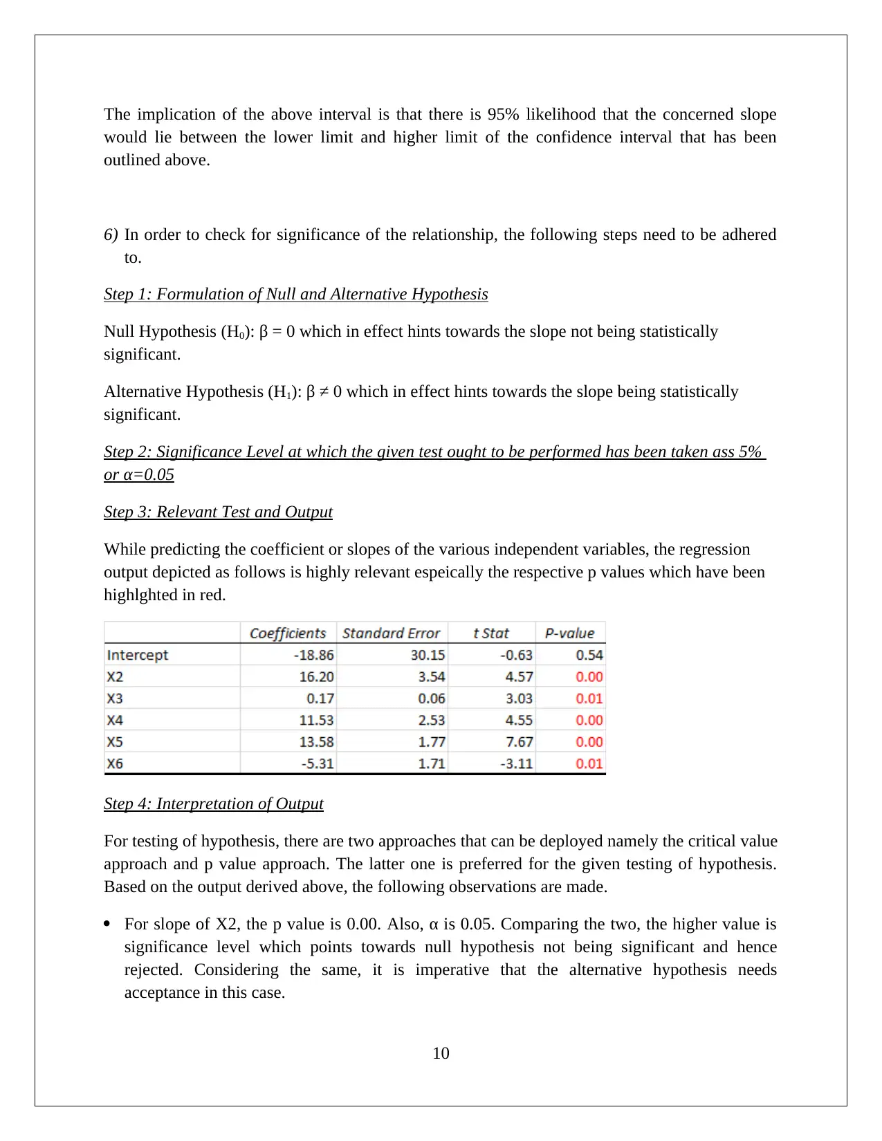
This assignment solution for HI6007 Statistics covers descriptive and inferential statistical analyses, focusing on startup costs and regression models. Task 1 involves calculating descriptive statistics, constructing frequency distributions and histograms, and conducting an ANOVA test to compare the average startup costs of different businesses. Task 2 utilizes regression analysis to model the relationship between annual sales and various independent variables, including franchise store area, inventory level, advertising spend, sales district families, and number of competing stores. The solution includes the formulation of hypotheses, significance level determination, test outputs, interpretation of results (including F-statistic and p-values), and conclusions. The interpretation of slope coefficients, confidence intervals, and the application of the regression model to predict annual sales are also provided, demonstrating a comprehensive understanding of statistical methods and their application in business contexts.

HI6007 STATISTICS
Student id
[Pick the date]

Task 1
1) The given question aims at various descriptive statistics related to central tendency and
dispersion. These have been computed by using inbuilt excel functions and the results thus
obtained are summarized in the tabular format illustrated below.
1

2) (a) The given class range is 0 to 30. Based on the instructions outlined in this regards, the
following frequency distribution tables for the startup costs of different businesses can be
obtained as has been represented.
(b) Considering the relative frequency table that have been plotted in part (a), the corresponding
histograms for each of the costs has been highlighted below.
2

3

4

3) Based on the output derived from part(1) and part (2), the following observations may be
drawn.
 Non-normal Distribution – The concerned variables do not highlight a normal
distribution which can be arrived from multiple evidences reflected above. The shape of
the concerned histogram is not symmetrical which signifies that skew presence is there.
Also, the mean along with median and mode do not settle at a single unified value for
either of the business which also imply the distribution not being normal.
 Difference in startup costs – The given sample through the mean tendency indicators and
also the histogram clearly reflect differences in the startup costs that are visible across
businesses. These potentially can be significant at the population level which needs to be
ascertained through the inferential statistical technique.
4) In order to check for difference in the average startup costs for the population of various given
businesses, the following steps need to be adhered to.
Step 1: Formulation of Null and Alternative Hypothesis
Null Hypothesis (H0): μX1= μX2= μX3= μX4= μX5
Alternative Hypothesis (H1): At a bare minimum, the startup costs on an average of one
particular business differes from the other startup costs on an average
Step 2: Significance Level at which the given test ought to be performed has been taken ass 5%
or α=0.05
Step 3: Relevant Test and Output
5

The test which would have to be applied here would be ANOVA and the output in this regards
has been taken from the MS=Excel regression output and reproduced below.
Step 4: Interpretation of Output
The critical aspect from the given output is F statistic which yields a value of 3.25. The
corresponding p value for the F statistic has comes out to be 0.02. This value needs to be
compared with the assumed level of significance. Comparing the two, the higher value is
significance level which points towards null hypothesis not being significant and hence rejected.
Step 5: Conclusion
On the basis of the output interpretation above, it would be appropriate to conclude that the
average startup costs for different businesses cannot be assumed to be same.
TASK 2
1) A useful tool available is MS-Excel under the Data Analysis option is the regression tool.
Using the data provided, this tool has been used for generating the output which has been
shared below.
6

The regression equation can be obtained using the value of the intercept along with the
coefficients derived for the various independent variables that are built into this model.
Independent Variable = x2, x3, x4, x5 & x6
Dependent Variable = x1
2) Fit is a key property of the regression model which tends to capture the underlying ability to
which the dependent variable movements can be accounted for or explained by the
corresponding variation of the independent variables on a joint basis. For a regression model,
it would be ideal that the fit is high or else there may be a need to introduce more predictors.
Two key parameters which are of significance in this regards are as follows.
 Coefficient of Determination – This value for the current regression model is quite
high at 0.9932 which can be opined considering that the highest possible magnitude is
1. The given value implies that 99.32% of dependent variable variation can be
accounted for by available independent variables in a collective manner.
 Model Significance – A key test for regression model significance is ANOVA which
is also available in the regression output that MS-Excel produces. This also reflects at
the statistically significant relation between the variables under consideration and
hence points towards a good fit.
7

3) In order to check for significance of the relationship, the following steps need to be adhered
to.
Step 1: Formulation of Null and Alternative Hypothesis
Null Hypothesis (H0): βX2= βX3= βX4= βX5= βX6=0
Alternative Hypothesis (H1): There is one slope at a minimum which would have non-zero slope
and hence reflect towards model significance
Step 2: Significance Level at which the given test ought to be performed has been taken ass 5%
or α=0.05
Step 3: Relevant Test and Output
The test which would have to be applied here would be ANOVA and the output in this regards
has been taken from the MS=Excel regression output and reproduced below.
Step 4: Interpretation of Output
The critical aspect from the given output is F statistic which yields a value of 611.59. The
corresponding p value for the F statistic has comes out to be 0.000. This value needs to be
compared with the assumed level of significance. Comparing the two, the higher value is
significance level which points towards null hypothesis not being significant and hence rejected.
Considering the same, it is imperative that the alternative hypothesis needs acceptance in this
case.
Step 5: Conclusion
On the basis of the output interpretation above, it would be appropriate to conclude that a
significant linear relation is existing between the variables of interest since all the regression
coefficients or slopes cannot be taken as zero.
4) For the interpretation of the slope coefficients, both their magnitude and direction would need
to be considered. The positive sign is indicative of the same directional change in independent
8

and concerned dependent variable. On the other hand, the negative sign is indicative of the
opposite directional change in the independent and concerned dependent variable. On the
other hand, the magnitude of the concerned slope hints towards the amount of change
expected to be seen in the independent variable on the unit change observed in the dependent
variable under consideration.
Based on the above broad guidelines, the interpretation of the slope coefficients obtained as part
of the regression model is given below.
 Variable – X2 (Slope Coefficient is 16.20) – The implication of this slope is that if there
is an increase or decrease in the area of the franchise store by 1 square feet, then the
corresponding change observed in the annual sales would be $ 16.20 is the direction of
change.
 Variable – X3 (Slope Coefficient is 0.17) - The implication of this slope is that if there is
an increase or decrease in the inventory of the franchise store by $1, then the
corresponding change observed in the annual sales would be $ 0.17 is the direction of
change.
 Variable – X4 (Slope Coefficient is 11.53) - The implication of this slope is that if there
is an increase or decrease in the amount of advertising spent by the franchise store by $1,
then the corresponding change observed in the annual sales would be $11.53 is the
direction of change.
 Variable – X5 (Slope Coefficient is 13.58) - The implication of this slope is that if there
is an increase or decrease in the amount of sales district by one family, then the
corresponding change observed in the annual sales would be $11.53 is the direction of
change.
 Variable – X6 (Slope Coefficient is -5.31) - The implication of this slope is that if there is
an increase or decrease in the competing stores in the corresponding district of the
franchise store by 1, then the corresponding change observed in the annual sales would
be $5,310 is the direction opposite to that of the change.
5) The confidence interval for the various slope coefficients that have been derived using the
output from the regression as has been indicated in the table attached below.
.
9

The implication of the above interval is that there is 95% likelihood that the concerned slope
would lie between the lower limit and higher limit of the confidence interval that has been
outlined above.
6) In order to check for significance of the relationship, the following steps need to be adhered
to.
Step 1: Formulation of Null and Alternative Hypothesis
Null Hypothesis (H0): β = 0 which in effect hints towards the slope not being statistically
significant.
Alternative Hypothesis (H1): β ≠ 0 which in effect hints towards the slope being statistically
significant.
Step 2: Significance Level at which the given test ought to be performed has been taken ass 5%
or α=0.05
Step 3: Relevant Test and Output
While predicting the coefficient or slopes of the various independent variables, the regression
output depicted as follows is highly relevant espeically the respective p values which have been
highlghted in red.
Step 4: Interpretation of Output
For testing of hypothesis, there are two approaches that can be deployed namely the critical value
approach and p value approach. The latter one is preferred for the given testing of hypothesis.
Based on the output derived above, the following observations are made.
 For slope of X2, the p value is 0.00. Also, α is 0.05. Comparing the two, the higher value is
significance level which points towards null hypothesis not being significant and hence
rejected. Considering the same, it is imperative that the alternative hypothesis needs
acceptance in this case.
10

 For slope of X3, the p value is 0.01. Also, α is 0.05. Comparing the two, the higher value is
significance level which points towards null hypothesis not being significant and hence
rejected. Considering the same, it is imperative that the alternative hypothesis needs
acceptance in this case.
 For slope of X4, the p value is 0.00. Also, α is 0.05. Comparing the two, the higher value is
significance level which points towards null hypothesis not being significant and hence
rejected. Considering the same, it is imperative that the alternative hypothesis needs
acceptance in this case.
 For slope of X5, the p value is 0.00. Also, α is 0.05. Comparing the two, the higher value is
significance level which points towards null hypothesis not being significant and hence
rejected. Considering the same, it is imperative that the alternative hypothesis needs
acceptance in this case.
 For slope of X6, the p value is 0.01. Also, α is 0.05. Comparing the two, the higher value is
significance level which points towards null hypothesis not being significant and hence
rejected. Considering the same, it is imperative that the alternative hypothesis needs
acceptance in this case.
Step 5: Conclusion
The interpretation of the above p value is indicative that various independent variables X2, X3,
X4, X5 & X6 are significant as it would not be prudent to assume any of the variables slope as
zero. Hence, each of the coefficients is significant for the explanation of the given dependent
variable.
7) In case any of the slopes would have failed to prove their significance, then alternations in the
regression model originally predicted would have been made. However, no changes are
suggested under the current scenario where it is apparent that all the independent variables are
of significance.
8) The model derived from part 1 would continue to be applied here in wake of the explanation
outlined in part 7. The relevant inputs are summarized below.
Area of the franchise store = 1,000 sq. ft and hence input is 1
Inventory level = $150,000 and hence input is 150
Spending on advertisement = $ 5,000 and hence input is 5
Families residing in the area of operation of the given franchise = 5000 and hence input is 5
Number of competing stores present in the area = 2
Using the above inputs and substituting the regression model predicted in part (1),
11

Annual sales (in 000’s) = -18.86 + 16.20*1+ 0.17*150 + 11.53*5 + 13.58*5 -5.31*2 = 138.448
Hence, the estimated annual sales for the given franchise store with attributed input values
should be about $ 138,448.
12