HI6007 Group Assignment: Statistical Analysis and Regression Models

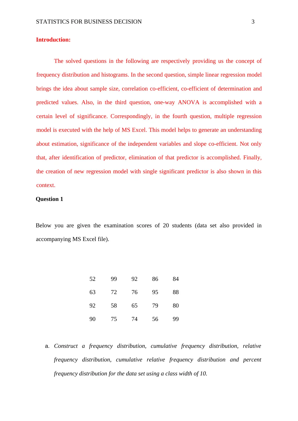
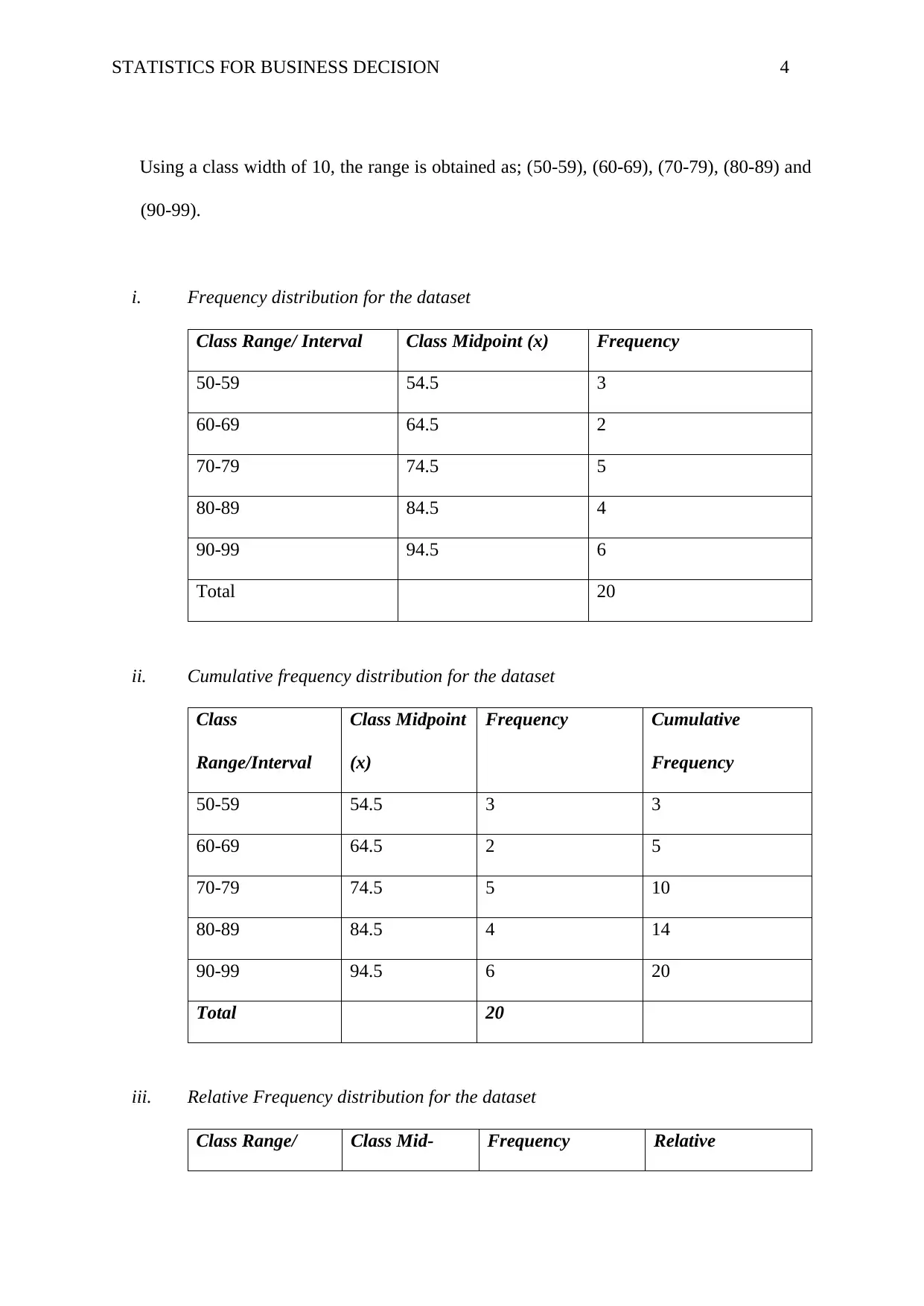
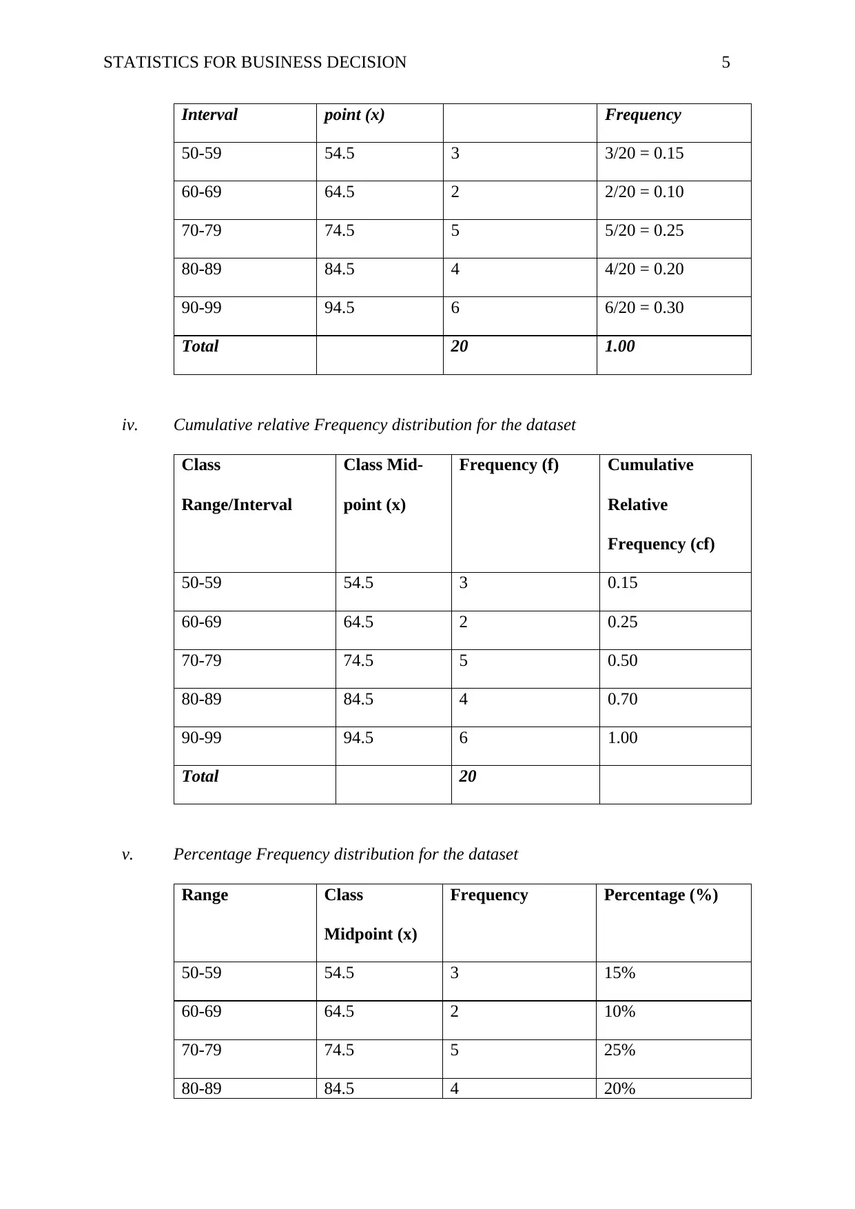
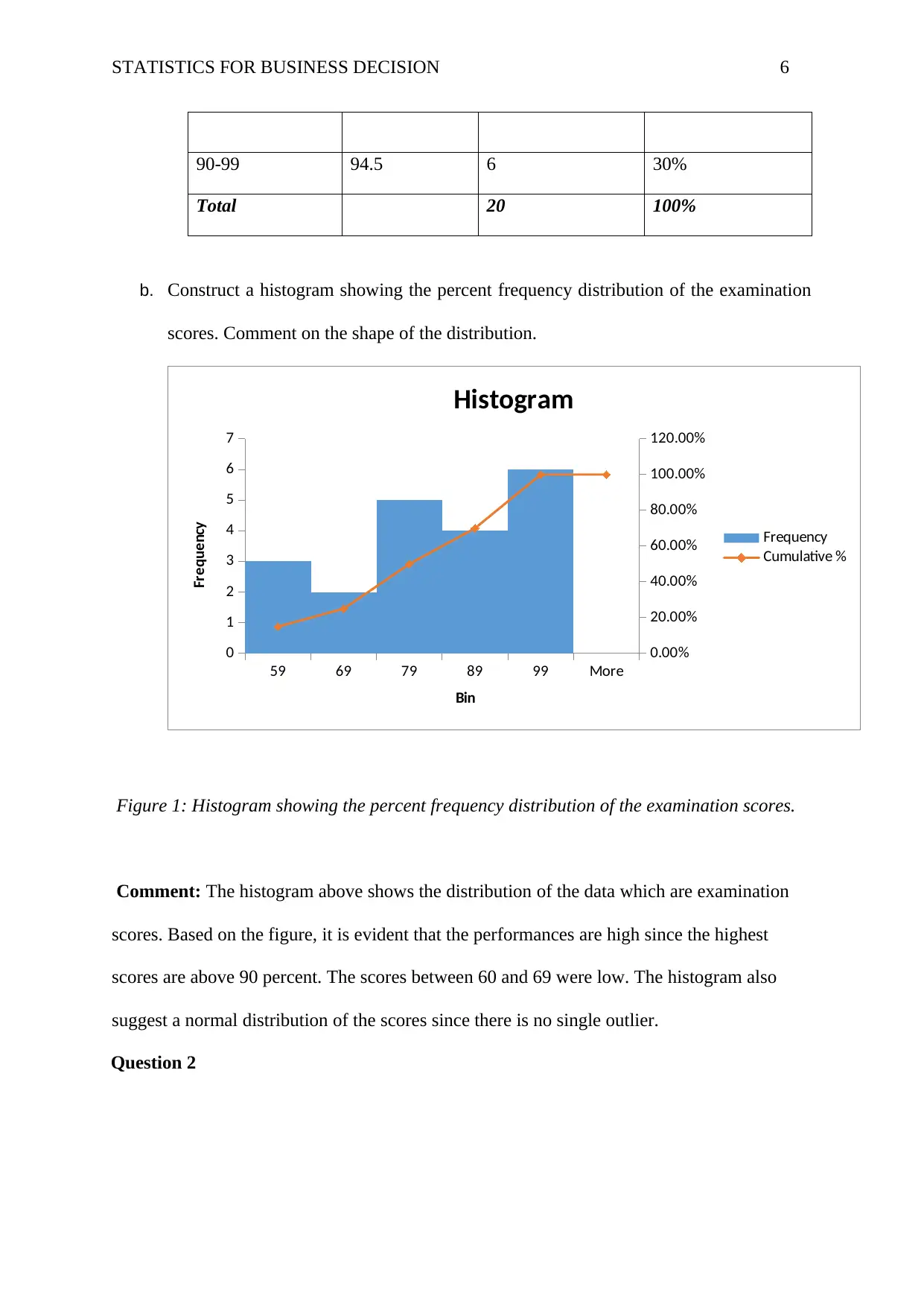
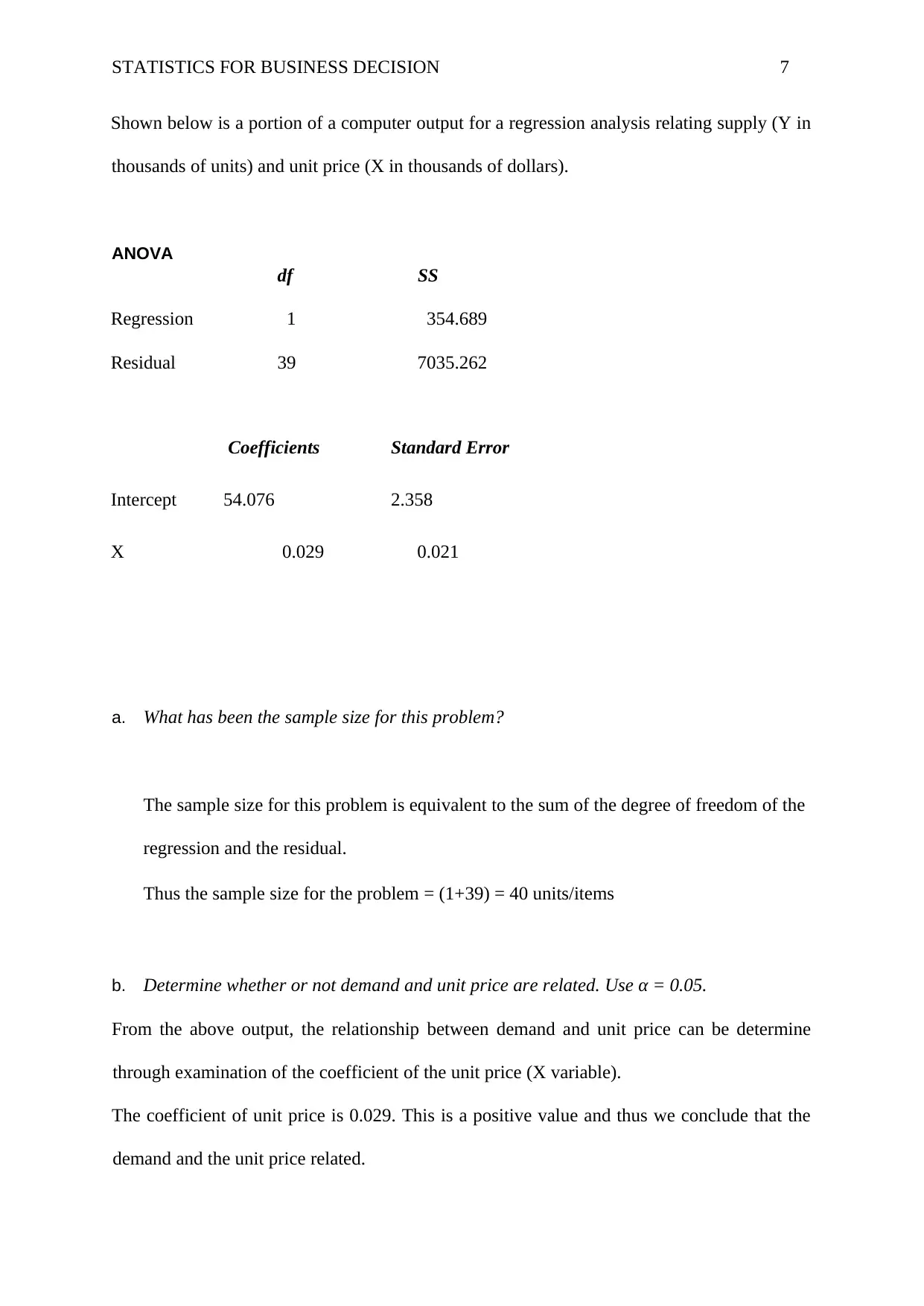
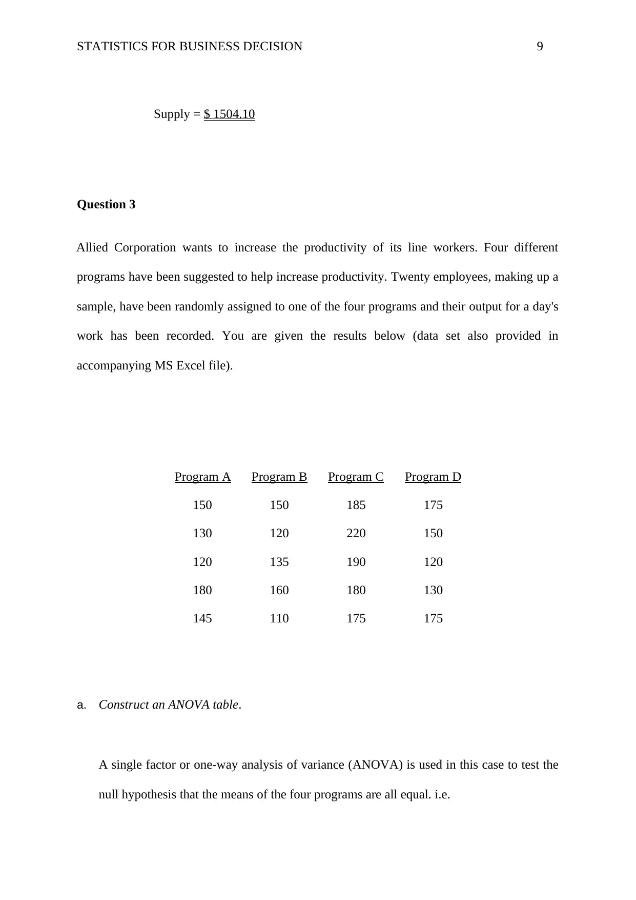
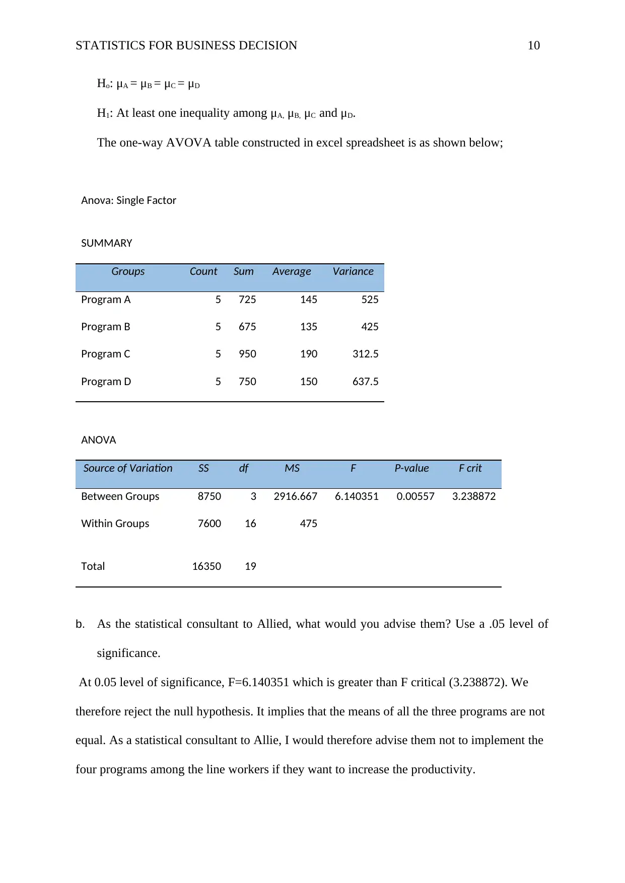
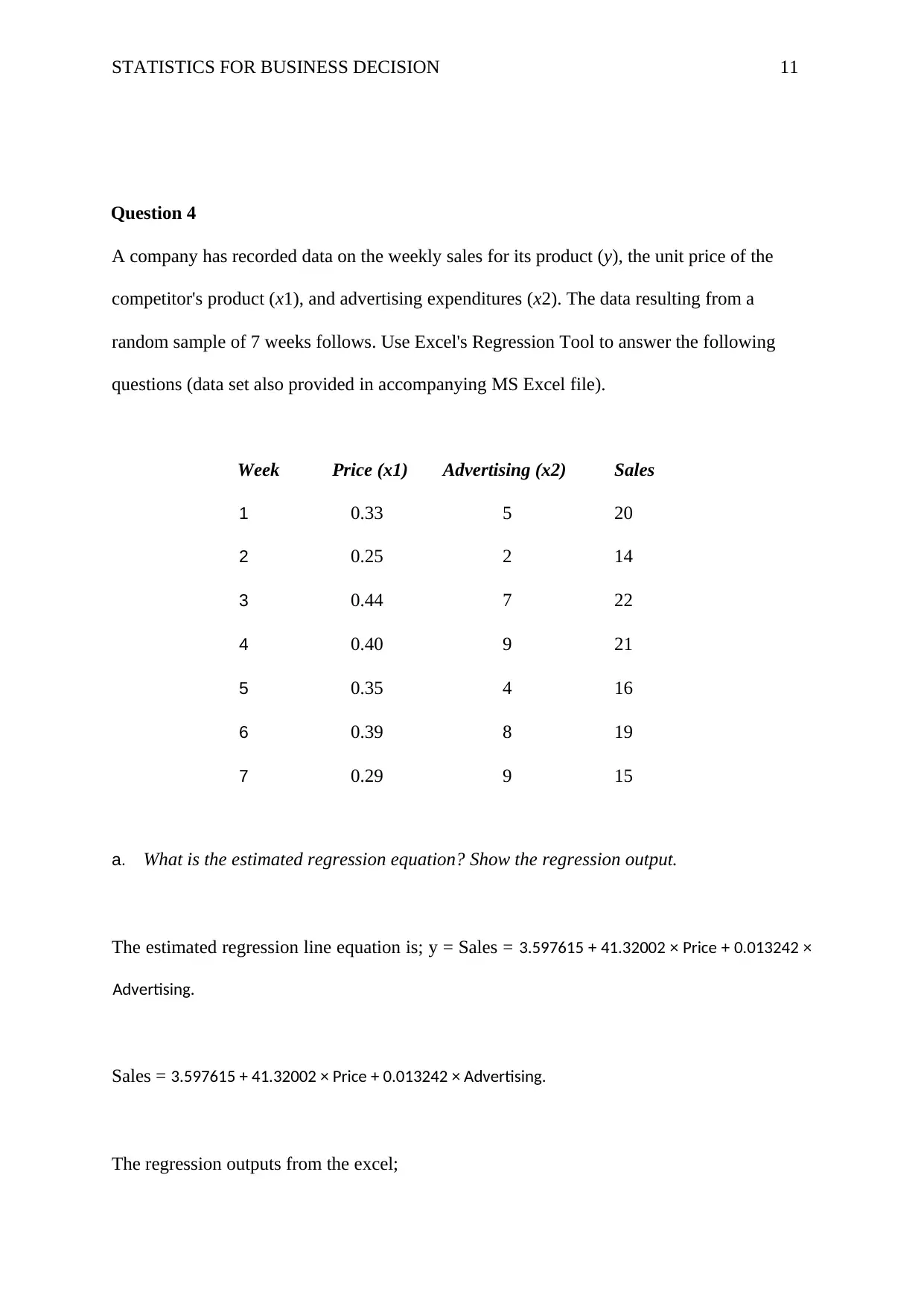
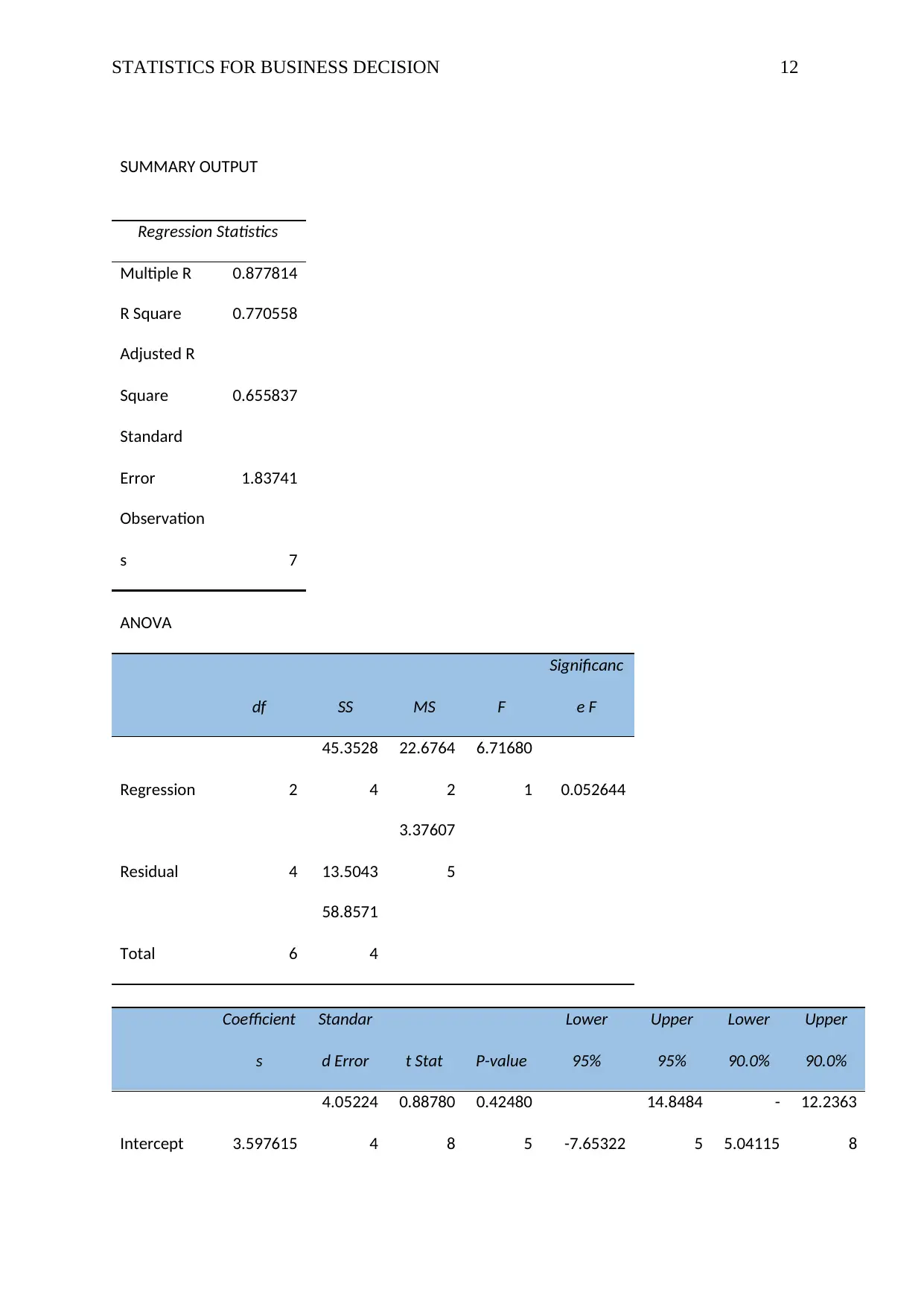
This assignment solution for HI6007 Statistics for Business Decisions covers several key statistical concepts. Question 1 focuses on constructing frequency distributions (frequency, cumulative frequency, relative frequency, cumulative relative frequency, and percentage frequency) and histograms from a dataset of examination scores, along with a comment on the distribution's shape. Question 2 delves into regression analysis, analyzing a computer output to determine the sample size, the relationship between demand and unit price, the coefficient of determination and correlation, and predicting supply based on unit price. Question 3 involves constructing an ANOVA table to assess the impact of different programs on worker productivity, followed by a recommendation. Finally, Question 4 uses Excel's Regression Tool to estimate a regression equation, assess its overall significance, determine the significance of individual variables, and re-estimate the model after dropping insignificant variables, including interpreting the slope coefficients.

Running head: STATISTICS FOR BUSINESS DECISION 1
HOLMES INSTITUTE FACULTY OF HIGHER EDUCATION
HI6007 Group Assignment
(Name of Student)
(University)
(Date of Submission)

STATISTICS FOR BUSINESS DECISION 2
Table of Contents
Introduction:............................................................................................................................. 3
Question 1................................................................................................................................ 3
Question 2................................................................................................................................ 7
Question 3................................................................................................................................ 9
Question 4.............................................................................................................................. 11
Conclusion:............................................................................................................................ 16
References............................................................................................................................. 17

STATISTICS FOR BUSINESS DECISION 3
Introduction:
The solved questions in the following are respectively providing us the concept of
frequency distribution and histograms. In the second question, simple linear regression model
brings the idea about sample size, correlation co-efficient, co-efficient of determination and
predicted values. Also, in the third question, one-way ANOVA is accomplished with a
certain level of significance. Correspondingly, in the fourth question, multiple regression
model is executed with the help of MS Excel. This model helps to generate an understanding
about estimation, significance of the independent variables and slope co-efficient. Not only
that, after identification of predictor, elimination of that predictor is accomplished. Finally,
the creation of new regression model with single significant predictor is also shown in this
context.
Question 1
Below you are given the examination scores of 20 students (data set also provided in
accompanying MS Excel file).
52 99 92 86 84
63 72 76 95 88
92 58 65 79 80
90 75 74 56 99
a. Construct a frequency distribution, cumulative frequency distribution, relative
frequency distribution, cumulative relative frequency distribution and percent
frequency distribution for the data set using a class width of 10.

STATISTICS FOR BUSINESS DECISION 4
Using a class width of 10, the range is obtained as; (50-59), (60-69), (70-79), (80-89) and
(90-99).
i. Frequency distribution for the dataset
Class Range/ Interval Class Midpoint (x) Frequency
50-59 54.5 3
60-69 64.5 2
70-79 74.5 5
80-89 84.5 4
90-99 94.5 6
Total 20
ii. Cumulative frequency distribution for the dataset
Class
Range/Interval
Class Midpoint
(x)
Frequency Cumulative
Frequency
50-59 54.5 3 3
60-69 64.5 2 5
70-79 74.5 5 10
80-89 84.5 4 14
90-99 94.5 6 20
Total 20
iii. Relative Frequency distribution for the dataset
Class Range/ Class Mid- Frequency Relative

STATISTICS FOR BUSINESS DECISION 5
Interval point (x) Frequency
50-59 54.5 3 3/20 = 0.15
60-69 64.5 2 2/20 = 0.10
70-79 74.5 5 5/20 = 0.25
80-89 84.5 4 4/20 = 0.20
90-99 94.5 6 6/20 = 0.30
Total 20 1.00
iv. Cumulative relative Frequency distribution for the dataset
Class
Range/Interval
Class Mid-
point (x)
Frequency (f) Cumulative
Relative
Frequency (cf)
50-59 54.5 3 0.15
60-69 64.5 2 0.25
70-79 74.5 5 0.50
80-89 84.5 4 0.70
90-99 94.5 6 1.00
Total 20
v. Percentage Frequency distribution for the dataset
Range Class
Midpoint (x)
Frequency Percentage (%)
50-59 54.5 3 15%
60-69 64.5 2 10%
70-79 74.5 5 25%
80-89 84.5 4 20%

STATISTICS FOR BUSINESS DECISION 6
90-99 94.5 6 30%
Total 20 100%
b. Construct a histogram showing the percent frequency distribution of the examination
scores. Comment on the shape of the distribution.
59 69 79 89 99 More
0
1
2
3
4
5
6
7
0.00%
20.00%
40.00%
60.00%
80.00%
100.00%
120.00%
Histogram
Frequency
Cumulative %
Bin
Frequency
Figure 1: Histogram showing the percent frequency distribution of the examination scores.
Comment: The histogram above shows the distribution of the data which are examination
scores. Based on the figure, it is evident that the performances are high since the highest
scores are above 90 percent. The scores between 60 and 69 were low. The histogram also
suggest a normal distribution of the scores since there is no single outlier.
Question 2

STATISTICS FOR BUSINESS DECISION 7
Shown below is a portion of a computer output for a regression analysis relating supply (Y in
thousands of units) and unit price (X in thousands of dollars).
ANOVA
df SS
Regression 1 354.689
Residual 39 7035.262
Coefficients Standard Error
Intercept 54.076 2.358
X 0.029 0.021
a. What has been the sample size for this problem?
The sample size for this problem is equivalent to the sum of the degree of freedom of the
regression and the residual.
Thus the sample size for the problem = (1+39) = 40 units/items
b. Determine whether or not demand and unit price are related. Use α = 0.05.
From the above output, the relationship between demand and unit price can be determine
through examination of the coefficient of the unit price (X variable).
The coefficient of unit price is 0.029. This is a positive value and thus we conclude that the
demand and the unit price related.

STATISTICS FOR BUSINESS DECISION 8
c. Compute the coefficient of determination and fully interpret its meaning. Be very specific.
The coefficient of determination helps in describing how well a regression line fits. i.e.
goodness of fit. Coefficient of determination (R²) is computed is computed based on the
following formula;
R² = 1- ∑ of Squares of Residuals
Total ∑ of Squares = 1- 7035.262
7389.951 = 0.047 which is approximately equals
to 0.
Given that the computed coefficient of determination = 0.047, it follows that the regression
line (line of best fit) does not fit the set of data points.
d. Compute the coefficient of correlation and explain the relationship between supply and
unit price.
The coefficient of determination (R²) is the square of the coefficient of the correlation ®.
But the coefficient of the determination computed in (c) above is 0.047.
Hence coefficient of correlation (R) = √Coefficient of determination
R = √0.047 = 0.2190
Based on the correlation of the coefficient computed which is 0.2190, this value is
positive and thus there exist a positive significant relationship/correlation between supply
and unit price.
d. Predict the supply (in units) when the unit price is $50,000.
The regression equation is; Supply (Y) = 54.076 + 0.029 × (50,000) + Standard error
Supply (Y) = 54.076 + 0.029 × (50,000) + 0.021

STATISTICS FOR BUSINESS DECISION 9
Supply = $ 1504.10
Question 3
Allied Corporation wants to increase the productivity of its line workers. Four different
programs have been suggested to help increase productivity. Twenty employees, making up a
sample, have been randomly assigned to one of the four programs and their output for a day's
work has been recorded. You are given the results below (data set also provided in
accompanying MS Excel file).
Program A Program B Program C Program D
150 150 185 175
130 120 220 150
120 135 190 120
180 160 180 130
145 110 175 175
a. Construct an ANOVA table.
A single factor or one-way analysis of variance (ANOVA) is used in this case to test the
null hypothesis that the means of the four programs are all equal. i.e.

STATISTICS FOR BUSINESS DECISION 10
Ho: μA = μB = μC = μD
H1: At least one inequality among μA, μB, μC and μD.
The one-way AVOVA table constructed in excel spreadsheet is as shown below;
Anova: Single Factor
SUMMARY
Groups Count Sum Average Variance
Program A 5 725 145 525
Program B 5 675 135 425
Program C 5 950 190 312.5
Program D 5 750 150 637.5
ANOVA
Source of Variation SS df MS F P-value F crit
Between Groups 8750 3 2916.667 6.140351 0.00557 3.238872
Within Groups 7600 16 475
Total 16350 19
b. As the statistical consultant to Allied, what would you advise them? Use a .05 level of
significance.
At 0.05 level of significance, F=6.140351 which is greater than F critical (3.238872). We
therefore reject the null hypothesis. It implies that the means of all the three programs are not
equal. As a statistical consultant to Allie, I would therefore advise them not to implement the
four programs among the line workers if they want to increase the productivity.

STATISTICS FOR BUSINESS DECISION 11
Question 4
A company has recorded data on the weekly sales for its product (y), the unit price of the
competitor's product (x1), and advertising expenditures (x2). The data resulting from a
random sample of 7 weeks follows. Use Excel's Regression Tool to answer the following
questions (data set also provided in accompanying MS Excel file).
Week Price (x1) Advertising (x2) Sales
1 0.33 5 20
2 0.25 2 14
3 0.44 7 22
4 0.40 9 21
5 0.35 4 16
6 0.39 8 19
7 0.29 9 15
a. What is the estimated regression equation? Show the regression output.
The estimated regression line equation is; y = Sales = 3.597615 + 41.32002 × Price + 0.013242 ×
Advertising.
Sales = 3.597615 + 41.32002 × Price + 0.013242 × Advertising.
The regression outputs from the excel;

STATISTICS FOR BUSINESS DECISION 12
SUMMARY OUTPUT
Regression Statistics
Multiple R 0.877814
R Square 0.770558
Adjusted R
Square 0.655837
Standard
Error 1.83741
Observation
s 7
ANOVA
df SS MS F
Significanc
e F
Regression 2
45.3528
4
22.6764
2
6.71680
1 0.052644
Residual 4 13.5043
3.37607
5
Total 6
58.8571
4
Coefficient
s
Standar
d Error t Stat P-value
Lower
95%
Upper
95%
Lower
90.0%
Upper
90.0%
Intercept 3.597615
4.05224
4
0.88780
8
0.42480
5 -7.65322
14.8484
5
-
5.04115
12.2363
8

STATISTICS FOR BUSINESS DECISION 13
Price (x1) 41.32002
13.3373
6
3.09806
5
0.03628
9 4.289567
78.3504
8
12.8868
1
69.7532
4
Advertising
(x2) 0.013242
0.32759
2
0.04042
2
0.96969
4 -0.8963
0.92278
2
-
0.68513
0.71161
7
RESIDUAL OUTPUT
Observatio
n
Predicted
Y
Residual
s
1 17.29943
2.70056
8
2 13.9541
0.04589
6
3 21.87112
0.12888
2
4 20.2448 0.7552
5 18.11259 -2.11259
6 19.81836 -0.81836
7 15.6996 -0.6996
b. Determine whether the model is significant overall. Use α = 0.10.
By using α = 0.10 as the level of significance, we interpret the overall F test of the
significance. We then compare the P-value for the F-test to our significance level. If the

STATISTICS FOR BUSINESS DECISION 14
P-value is less than the significance level, then the sample data would provide a sufficient
evidence to conclude that the regression model is significant.
In our case, the P-value= 0.424805 which is greater than the significance level (α = 0.10).
Thus the overall model is not significant.
c. Determine if competitor’s price and advertising is individually significantly related to
sales. Use α = 0.10.
Statistical significant is the likelihood that the relationship between competitor’s price and
advertising is related to sales. The P-value is examined to determine if competitor’s price and
advertising is individually significantly related to sales. If the P- value obtained in each
variable is lower than 5% i.e. 0.05, then the variable is individually significantly related to
sales. In this case, the P-value under competitor’s price is 0.036289 while that of advertising is
0.969694. It implies that only competitor’s price is individually significantly related to sales since its
P- value is less than 0. 05. Thus, advertising is an insignificant variable.
d. Based on your answer to part (c), drop any insignificant independent variable(s) and d.
Re-estimate the model. What is the new estimated regression equation?
Based on the findings, the advertising is the insignificant independent variable to be
dropped since it has a P-value that is higher than 5 percent (0.05). We then res-estimate
the model and the new estimated regression equation becomes; Sales = 3.581788 +
41.60305 × Competitor’s Price
The new estimated regression equation;

STATISTICS FOR BUSINESS DECISION 15
Sales = 3.581788 + 41.60305 × Competitor’s Price
Excel output is as shown below.
SUMMARY OUTPUT
Regression Statistics
Multiple R
0.87776
1
R Square
0.77046
4
Adjusted R
Square
0.72455
7
Standard
Error
1.64376
5
Observation
s 7
ANOVA
df SS MS F
Significa
nce F
Regression 1 45.34733
45.34
733
16.78
311 0.009385
Residual 5 13.50981
2.701
963
Total 6 58.85714
Coeffici Standard t Stat P- Lower Upper Lower Upper

STATISTICS FOR BUSINESS DECISION 16
ents Error value 95% 95% 90.0% 90.0%
Intercept
3.58178
8 3.608215
0.992
676
0.366
447 -5.69342 12.857 -3.68894
10.8525
2
Price (x1)
41.6030
5 10.15521
4.096
719
0.009
385 15.49825
67.707
86
21.1398
1 62.0663
d. Interpret the slope coefficient(s) of the model from part (d).
From the model obtained above the coefficient of competitor’s price is obtained as 41.60305.
It therefore follows that for each unit increase in competitor’s price, the value of sale
increases with a value that is equivalent to 41.60305.
Conclusion:
Finally, the questions of the assignment help to create a transparent concept about
using common MS Excel functions and ‘Data analysis’ tool-pack. The approach of
distribution and its aspects of any continuous variable (ex: exam scores of the students) is
analyzed as well as depicted with respect to the analytical report. The interrelationship of
various statistics and parameters of linear regression model or multiple regression model are
learned in this analytical report. The ANOVA test taught us about rejecting or accepting the
null or alternative hypothesis with respect to certain level of significance (here 5%). The
strength of association and its significance as per coefficient of correlation or coefficient of
determination are established with the reference of regression analysis. The estimation or
prediction approach is apprehended by the simple or multiple regression models.

STATISTICS FOR BUSINESS DECISION 17
References
John, A. Rice (2005).Mathematical Statistics and Data Analysis. Berkeley: University of
California
Gulezian, R. (2006). Elements of Business Statistics. London: Oxford press