Statistics and Research Methodology: Hypothesis Testing and Analysis

This document presents a comprehensive solution to a statistics and research methodology assignment, encompassing a range of statistical techniques. It includes detailed explanations and calculations for various hypothesis tests, such as one-sample t-tests, independent sample t-tests, and t-tests for differences of population means. The assignment also covers analysis of variance (ANOVA) to compare multiple groups and regression analysis to assess relationships between variables. Furthermore, the solutions address practical applications, including analyzing customer data, comparing firm performance, and predicting delivery times. The document demonstrates the application of these statistical methods to real-world scenarios, providing insights into data analysis and interpretation. The assignment covers concepts such as null and alternate hypothesis, degrees of freedom, p-values, and the interpretation of statistical results. The document serves as a valuable resource for students seeking to understand and apply statistical methods in research and analysis.

Running Head: STATISTICS AND RESEARCH METHODOLOGY
Statistics and Research Methodology
Name of the Student
Name of the University
Author Note

1STATISTICS AND RESEARCH METHODOLOGY
Table of Contents
Answer 1..........................................................................................................................................2
Answer 2..........................................................................................................................................3
Answer 3..........................................................................................................................................5
Answer 4..........................................................................................................................................5
Answer 5..........................................................................................................................................6
Answer 6..........................................................................................................................................8
Answer 7..........................................................................................................................................8
Answer 8..........................................................................................................................................9
Answer 9........................................................................................................................................10
Answer 10......................................................................................................................................11
Answer 11......................................................................................................................................13

2STATISTICS AND RESEARCH METHODOLOGY
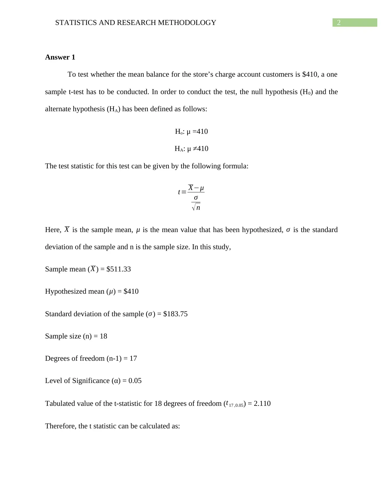
Answer 1
To test whether the mean balance for the store’s charge account customers is $410, a one
sample t-test has to be conducted. In order to conduct the test, the null hypothesis (H0) and the
alternate hypothesis (HA) has been defined as follows:
Ho: μ =410
HA: μ ≠410
The test statistic for this test can be given by the following formula:
t= X−μ
σ
√ n
Here, X is the sample mean, μ is the mean value that has been hypothesized, σ is the standard
deviation of the sample and n is the sample size. In this study,
Sample mean ( X ) = $511.33
Hypothesized mean ( μ) = $410
Standard deviation of the sample ( σ ) = $183.75
Sample size (n) = 18
Degrees of freedom (n-1) = 17
Level of Significance (α) = 0.05
Tabulated value of the t-statistic for 18 degrees of freedom ( t17 ,0.05) = 2.110
Therefore, the t statistic can be calculated as:

3STATISTICS AND RESEARCH METHODOLOGY
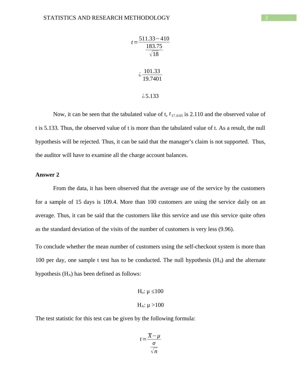
t= 511.33−410
183.75
√ 18
¿ 101.33
19.7401
¿ 5.133
Now, it can be seen that the tabulated value of t, t17 ,0.05 is 2.110 and the observed value of
t is 5.133. Thus, the observed value of t is more than the tabulated value of t. As a result, the null
hypothesis will be rejected. Thus, it can be said that the manager’s claim is not supported. Thus,
the auditor will have to examine all the charge account balances.
Answer 2
From the data, it has been observed that the average use of the service by the customers
for a sample of 15 days is 109.4. More than 100 customers are using the service daily on an
average. Thus, it can be said that the customers like this service and use this service quite often
as the standard deviation of the visits of the number of customers is very less (9.96).
To conclude whether the mean number of customers using the self-checkout system is more than
100 per day, one sample t test has to be conducted. The null hypothesis (H0) and the alternate
hypothesis (HA) has been defined as follows:
Ho: μ ≤100
HA: μ >100
The test statistic for this test can be given by the following formula:
t= X−μ
σ
√ n

4STATISTICS AND RESEARCH METHODOLOGY
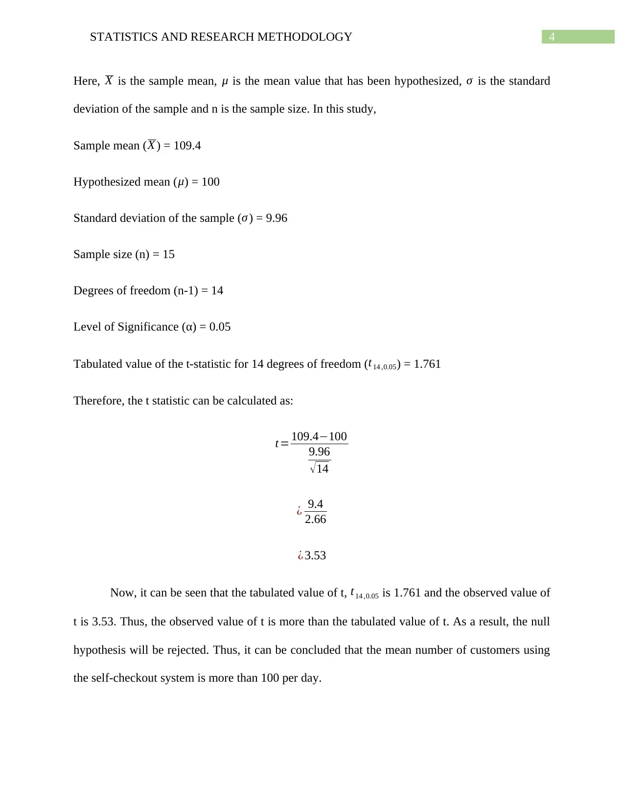
Here, X is the sample mean, μ is the mean value that has been hypothesized, σ is the standard
deviation of the sample and n is the sample size. In this study,
Sample mean ( X ) = 109.4
Hypothesized mean ( μ) = 100
Standard deviation of the sample ( σ ) = 9.96
Sample size (n) = 15
Degrees of freedom (n-1) = 14
Level of Significance (α) = 0.05
Tabulated value of the t-statistic for 14 degrees of freedom ( t14 ,0.05) = 1.761
Therefore, the t statistic can be calculated as:
t= 109.4−100
9.96
√ 14
¿ 9.4
2.66
¿ 3.53
Now, it can be seen that the tabulated value of t, t14 ,0.05 is 1.761 and the observed value of
t is 3.53. Thus, the observed value of t is more than the tabulated value of t. As a result, the null
hypothesis will be rejected. Thus, it can be concluded that the mean number of customers using
the self-checkout system is more than 100 per day.

5STATISTICS AND RESEARCH METHODOLOGY
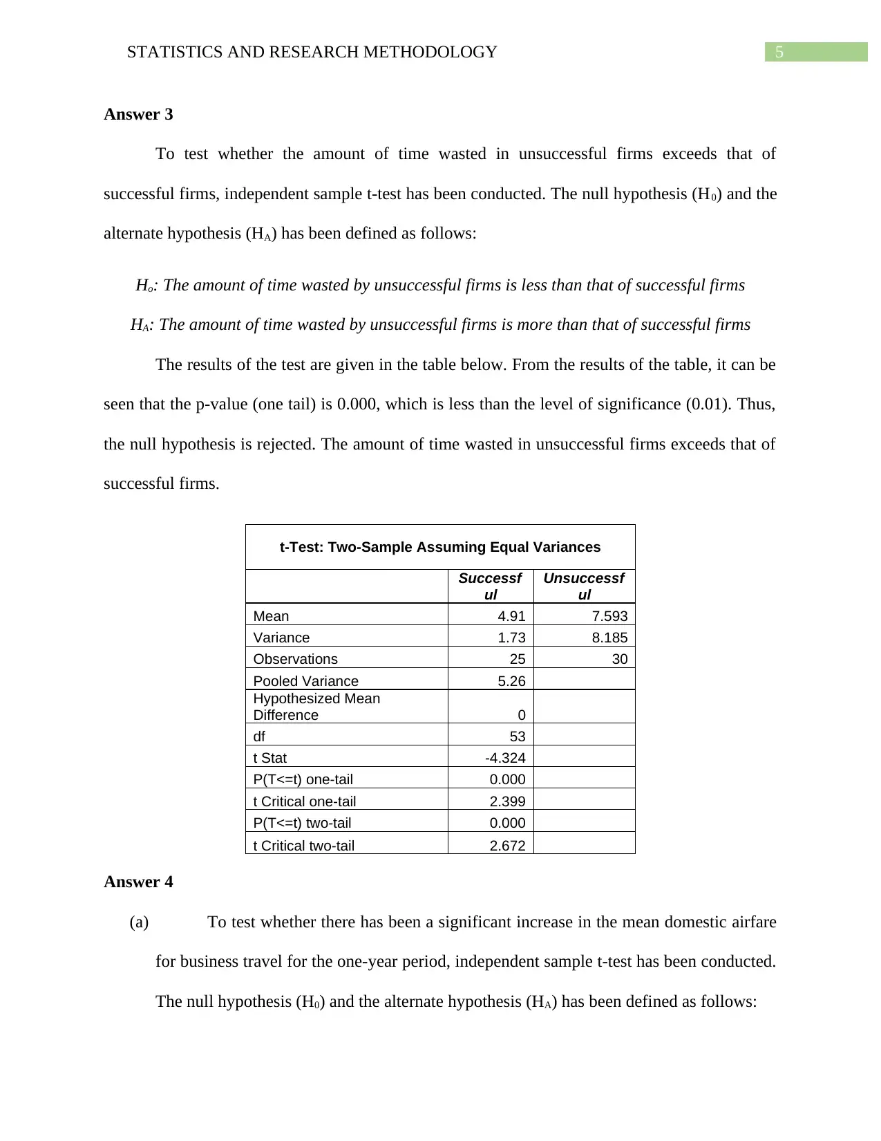
Answer 3
To test whether the amount of time wasted in unsuccessful firms exceeds that of
successful firms, independent sample t-test has been conducted. The null hypothesis (H0) and the
alternate hypothesis (HA) has been defined as follows:
Ho: The amount of time wasted by unsuccessful firms is less than that of successful firms
HA: The amount of time wasted by unsuccessful firms is more than that of successful firms
The results of the test are given in the table below. From the results of the table, it can be
seen that the p-value (one tail) is 0.000, which is less than the level of significance (0.01). Thus,
the null hypothesis is rejected. The amount of time wasted in unsuccessful firms exceeds that of
successful firms.
t-Test: Two-Sample Assuming Equal Variances
Successf
ul
Unsuccessf
ul
Mean 4.91 7.593
Variance 1.73 8.185
Observations 25 30
Pooled Variance 5.26
Hypothesized Mean
Difference 0
df 53
t Stat -4.324
P(T<=t) one-tail 0.000
t Critical one-tail 2.399
P(T<=t) two-tail 0.000
t Critical two-tail 2.672
Answer 4
(a) To test whether there has been a significant increase in the mean domestic airfare
for business travel for the one-year period, independent sample t-test has been conducted.
The null hypothesis (H0) and the alternate hypothesis (HA) has been defined as follows:

6STATISTICS AND RESEARCH METHODOLOGY
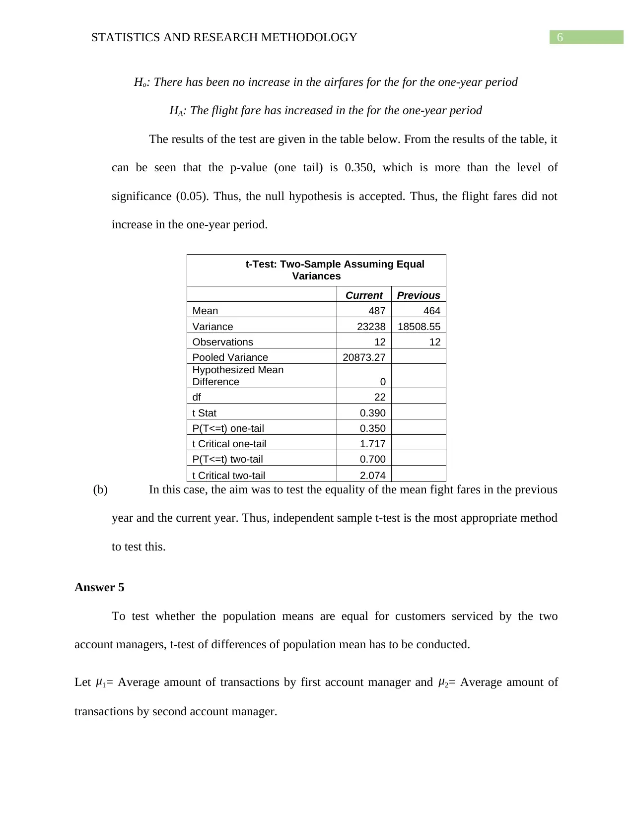
Ho: There has been no increase in the airfares for the for the one-year period
HA: The flight fare has increased in the for the one-year period
The results of the test are given in the table below. From the results of the table, it
can be seen that the p-value (one tail) is 0.350, which is more than the level of
significance (0.05). Thus, the null hypothesis is accepted. Thus, the flight fares did not
increase in the one-year period.
t-Test: Two-Sample Assuming Equal
Variances
Current Previous
Mean 487 464
Variance 23238 18508.55
Observations 12 12
Pooled Variance 20873.27
Hypothesized Mean
Difference 0
df 22
t Stat 0.390
P(T<=t) one-tail 0.350
t Critical one-tail 1.717
P(T<=t) two-tail 0.700
t Critical two-tail 2.074
(b) In this case, the aim was to test the equality of the mean fight fares in the previous
year and the current year. Thus, independent sample t-test is the most appropriate method
to test this.
Answer 5
To test whether the population means are equal for customers serviced by the two
account managers, t-test of differences of population mean has to be conducted.
Let μ1= Average amount of transactions by first account manager and μ2= Average amount of
transactions by second account manager.

7STATISTICS AND RESEARCH METHODOLOGY
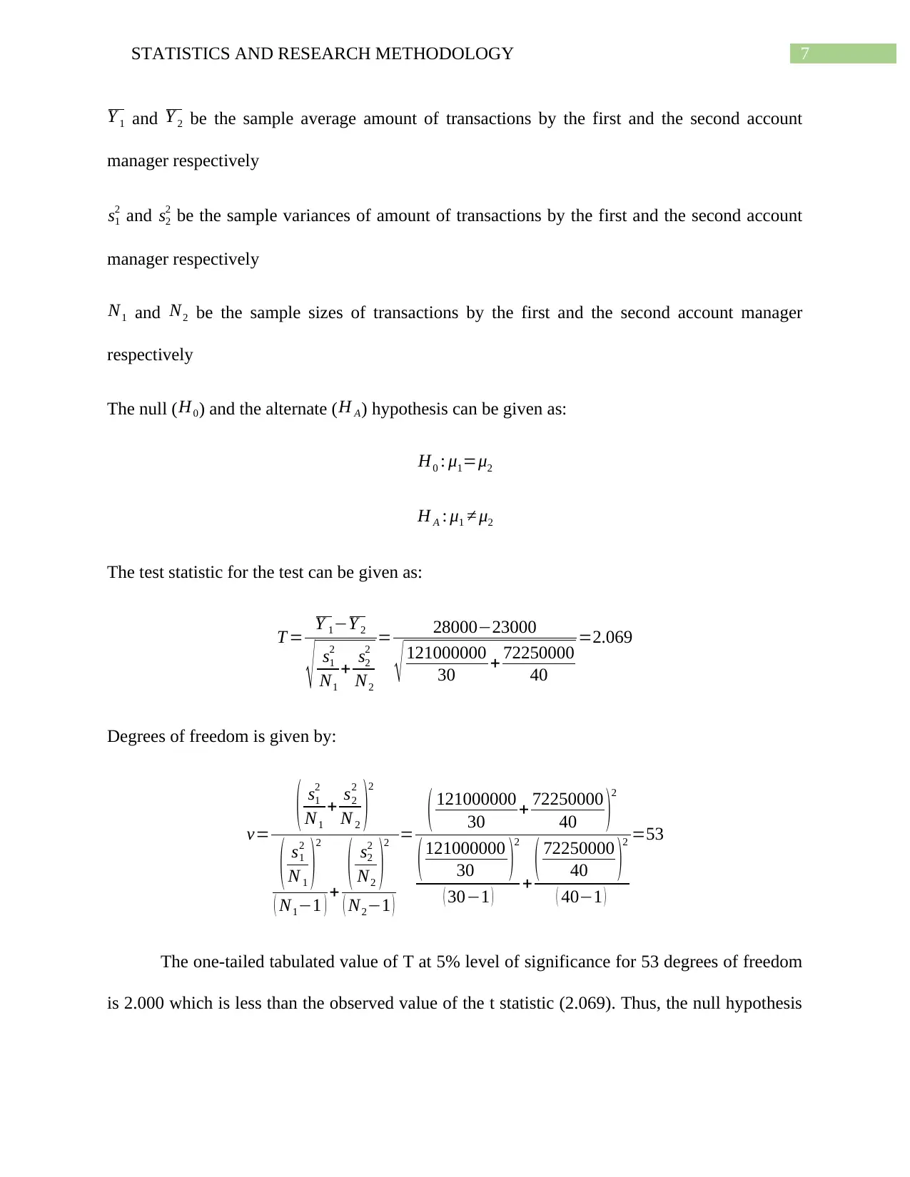
Y 1 and Y 2 be the sample average amount of transactions by the first and the second account
manager respectively
s1
2 and s2
2 be the sample variances of amount of transactions by the first and the second account
manager respectively
N1 and N2 be the sample sizes of transactions by the first and the second account manager
respectively
The null ( H0) and the alternate ( H A) hypothesis can be given as:
H0 : μ1=μ2
H A : μ1 ≠ μ2
The test statistic for the test can be given as:
T = Y 1−Y 2
√ s1
2
N1
+ s2
2
N2
= 28000−23000
√ 121000000
30 + 72250000
40
=2.069
Degrees of freedom is given by:
v=
( s1
2
N1
+ s2
2
N 2 )2
( s1
2
N 1 )2
( N1−1 ) +
( s2
2
N2 )2
( N2−1 )
= ( 121000000
30 + 72250000
40 )2
(121000000
30 )2
( 30−1 ) + ( 72250000
40 )2
( 40−1 )
=53
The one-tailed tabulated value of T at 5% level of significance for 53 degrees of freedom
is 2.000 which is less than the observed value of the t statistic (2.069). Thus, the null hypothesis

8STATISTICS AND RESEARCH METHODOLOGY
is rejected. Thus, it can be said that the population means are not equal for customers serviced by
the two account managers.
Answer 6
(a) To test the differences in the job satisfaction among the three professions, one-
way analysis of variance (ANOVA) test has been conducted. The null hypothesis (H0)
and the alternate hypothesis (HA) has been defined as follows:
Ho: There has been no differences in the job satisfaction among the three professions
HA: There is significant difference in the job satisfaction among the three professions
From the test results, it can be seen that, the p-value is 0.04 which is less than the
level of significance (0.05). Thus, the null hypothesis is rejected. There are significant
differences in the job satisfaction of different types of professions.
(b) The ANOVA test only signifies whether there is any significant difference
between a number of groups. But the difference between which two groups has created
this discrepancy cannot be understood from the ANOVA test. Thus, Tukey Test is to be
performed. From the results of the Tukey test, it has been seen that the value of the q stat
for the pair of variables Systems Analysts and Lawyers is more than the critical value of
the q statistic for 27 degrees of freedom for three groups. Thus, difference exists between
Systems Analysts and Lawyers.
Answer 7
(a) To test whether the speed of promotion varies between the three sizes of
engineering firms, one-way analysis of variance (ANOVA) test has been conducted.
From the results of the analysis it has been observed that the p-value is 0.029 which is

9STATISTICS AND RESEARCH METHODOLOGY
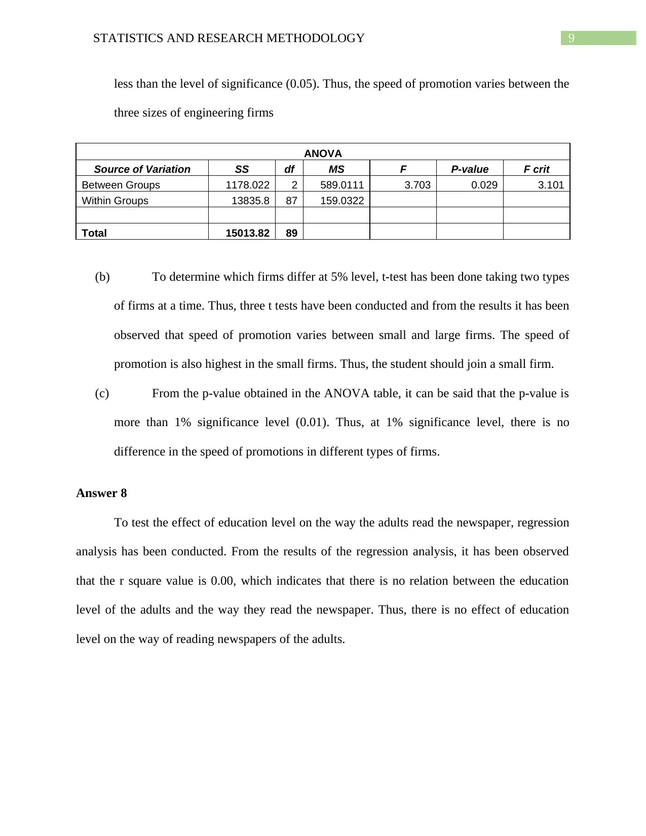
less than the level of significance (0.05). Thus, the speed of promotion varies between the
three sizes of engineering firms
ANOVA
Source of Variation SS df MS F P-value F crit
Between Groups 1178.022 2 589.0111 3.703 0.029 3.101
Within Groups 13835.8 87 159.0322
Total 15013.82 89
(b) To determine which firms differ at 5% level, t-test has been done taking two types
of firms at a time. Thus, three t tests have been conducted and from the results it has been
observed that speed of promotion varies between small and large firms. The speed of
promotion is also highest in the small firms. Thus, the student should join a small firm.
(c) From the p-value obtained in the ANOVA table, it can be said that the p-value is
more than 1% significance level (0.01). Thus, at 1% significance level, there is no
difference in the speed of promotions in different types of firms.
Answer 8
To test the effect of education level on the way the adults read the newspaper, regression
analysis has been conducted. From the results of the regression analysis, it has been observed
that the r square value is 0.00, which indicates that there is no relation between the education
level of the adults and the way they read the newspaper. Thus, there is no effect of education
level on the way of reading newspapers of the adults.

10STATISTICS AND RESEARCH METHODOLOGY
Answer 9
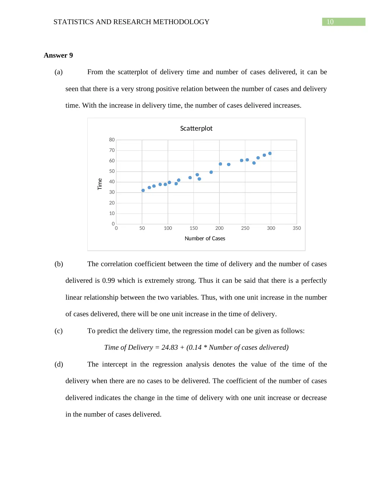
(a) From the scatterplot of delivery time and number of cases delivered, it can be
seen that there is a very strong positive relation between the number of cases and delivery
time. With the increase in delivery time, the number of cases delivered increases.
0 50 100 150 200 250 300 350
0
10
20
30
40
50
60
70
80
Scatterplot
Number of Cases
Time
(b) The correlation coefficient between the time of delivery and the number of cases
delivered is 0.99 which is extremely strong. Thus it can be said that there is a perfectly
linear relationship between the two variables. Thus, with one unit increase in the number
of cases delivered, there will be one unit increase in the time of delivery.
(c) To predict the delivery time, the regression model can be given as follows:
Time of Delivery = 24.83 + (0.14 * Number of cases delivered)
(d) The intercept in the regression analysis denotes the value of the time of the
delivery when there are no cases to be delivered. The coefficient of the number of cases
delivered indicates the change in the time of delivery with one unit increase or decrease
in the number of cases delivered.

11STATISTICS AND RESEARCH METHODOLOGY
(e) The coefficient of determination in this problem is 0.99 which indicates that the
99 percent of the variation in the time of delivery can be explained by the number of
cases to be delivered.
(f) The p-values of the regression coefficients are less than the 5% level of
significance (0.05). Thus, the variables are significant to the model. This indicates that
there is a linear relationship between the time of delivery and the number of cases
delivered.
(g) The delivery time for 150 cases of soft drink is
Time of Delivery = 24.83 + (0.14 * 150) = 45.83
(h) There is 95% confidence that the mean delivery time for 150 cases of soft drink is
45.83 minutes.
(i) There is 95% confidence that the delivery time for a single delivery of 150 cases
of soft drink is 45.83 minutes.
(j) The model cannot be used to predict the delivery time for a customer who is
receiving 500 cases of soft drink because regression is used to predict any values within
the given range of values. 500 cases is outside the given range of values. Thus, this model
cannot be used to predict the time of delivery of 500 cases.
(k) To deliver 200 cases, the time required will be
Time of Delivery = 24.83 + (0.14 * 200) = 52.83 minutes.
Thus, the claim maid by the manager is not accurate.