HI6007 Statistics and Research Methods Group Assignment T2 2019

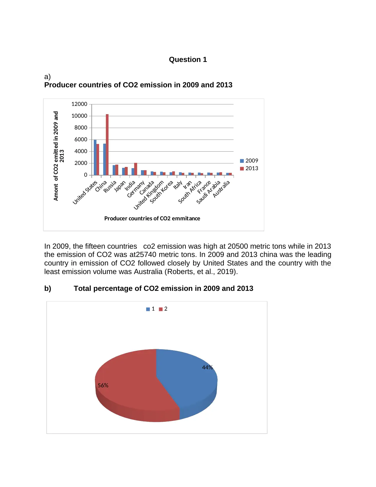
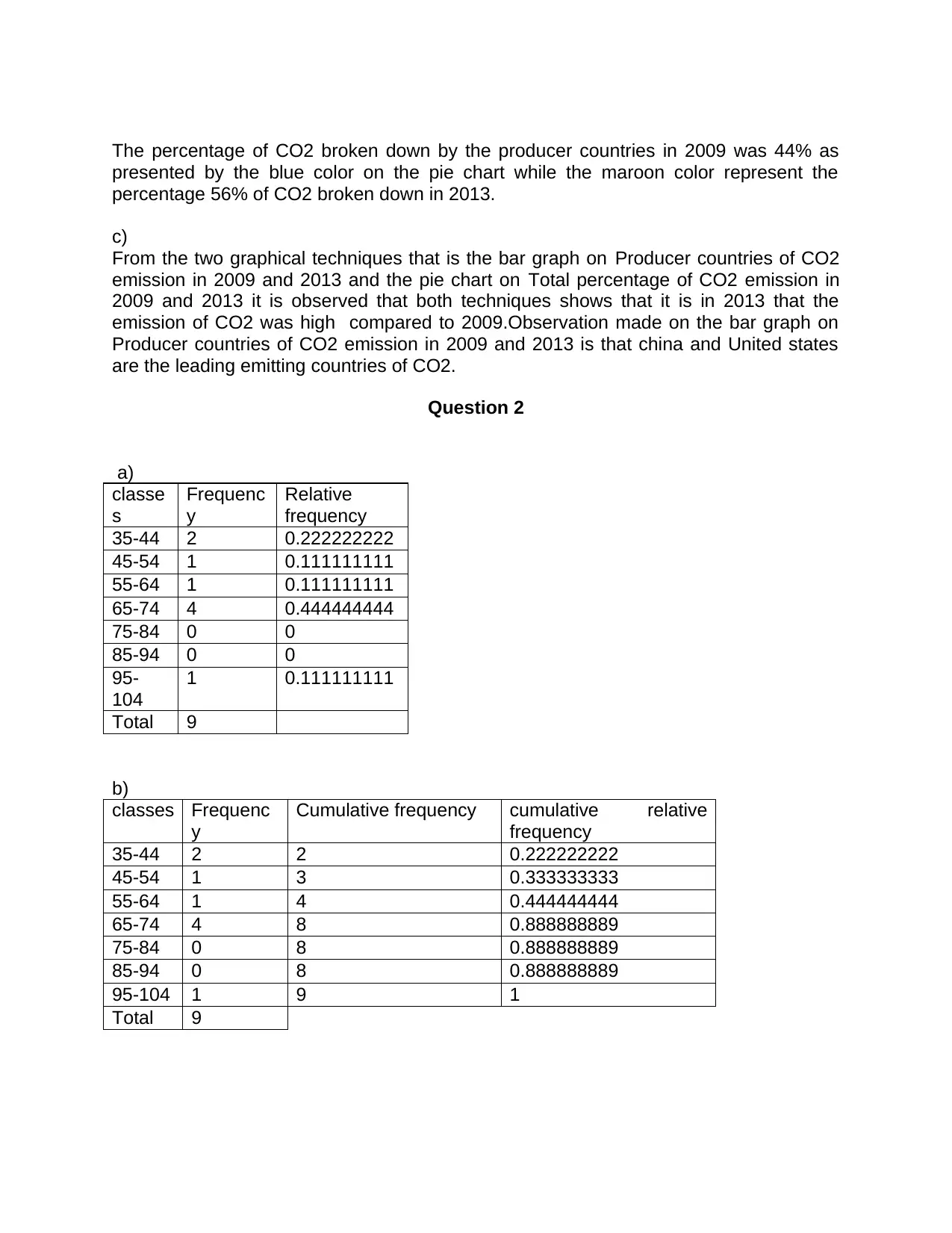
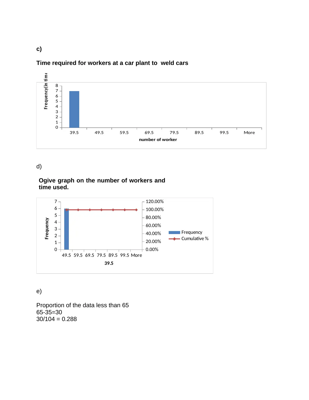
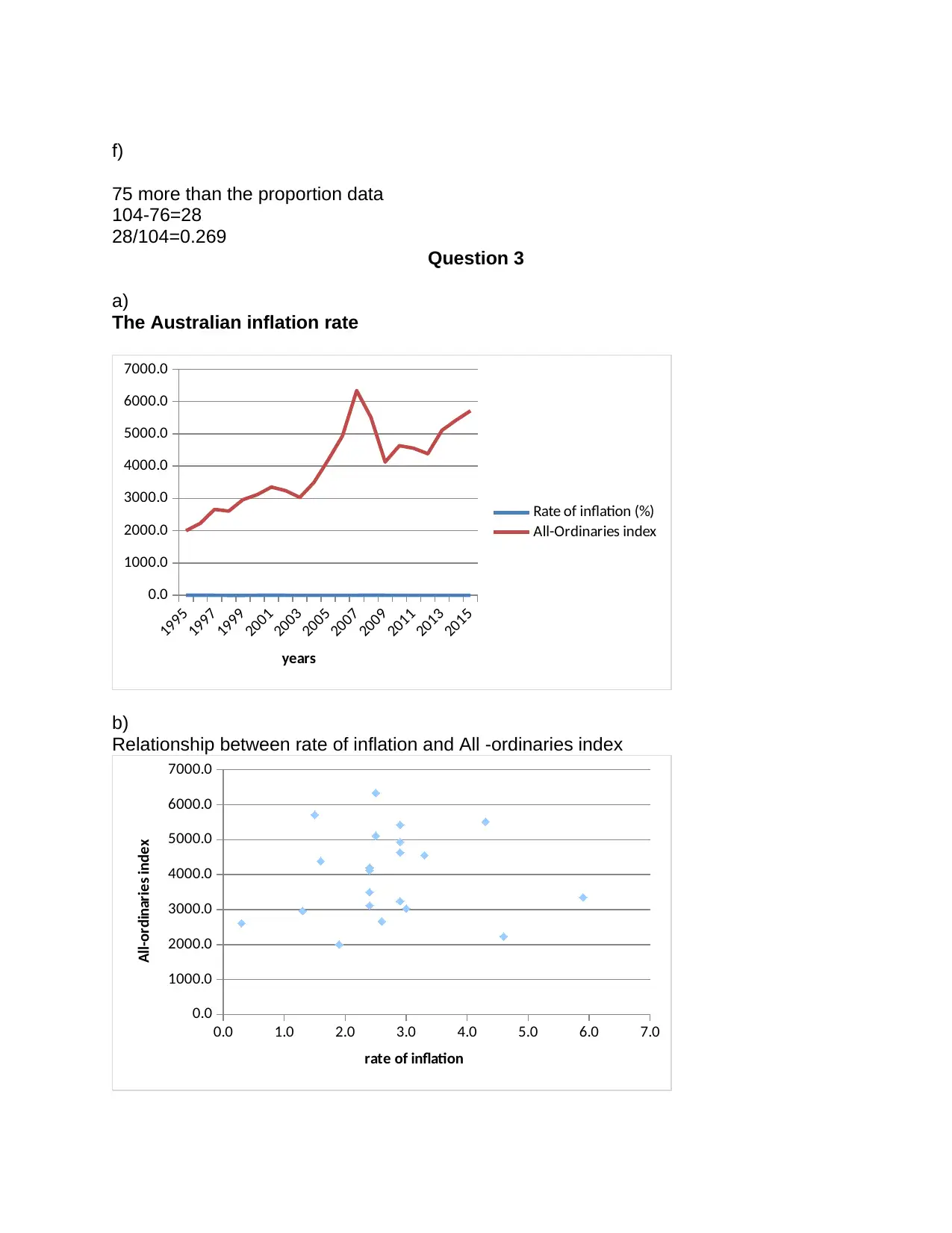
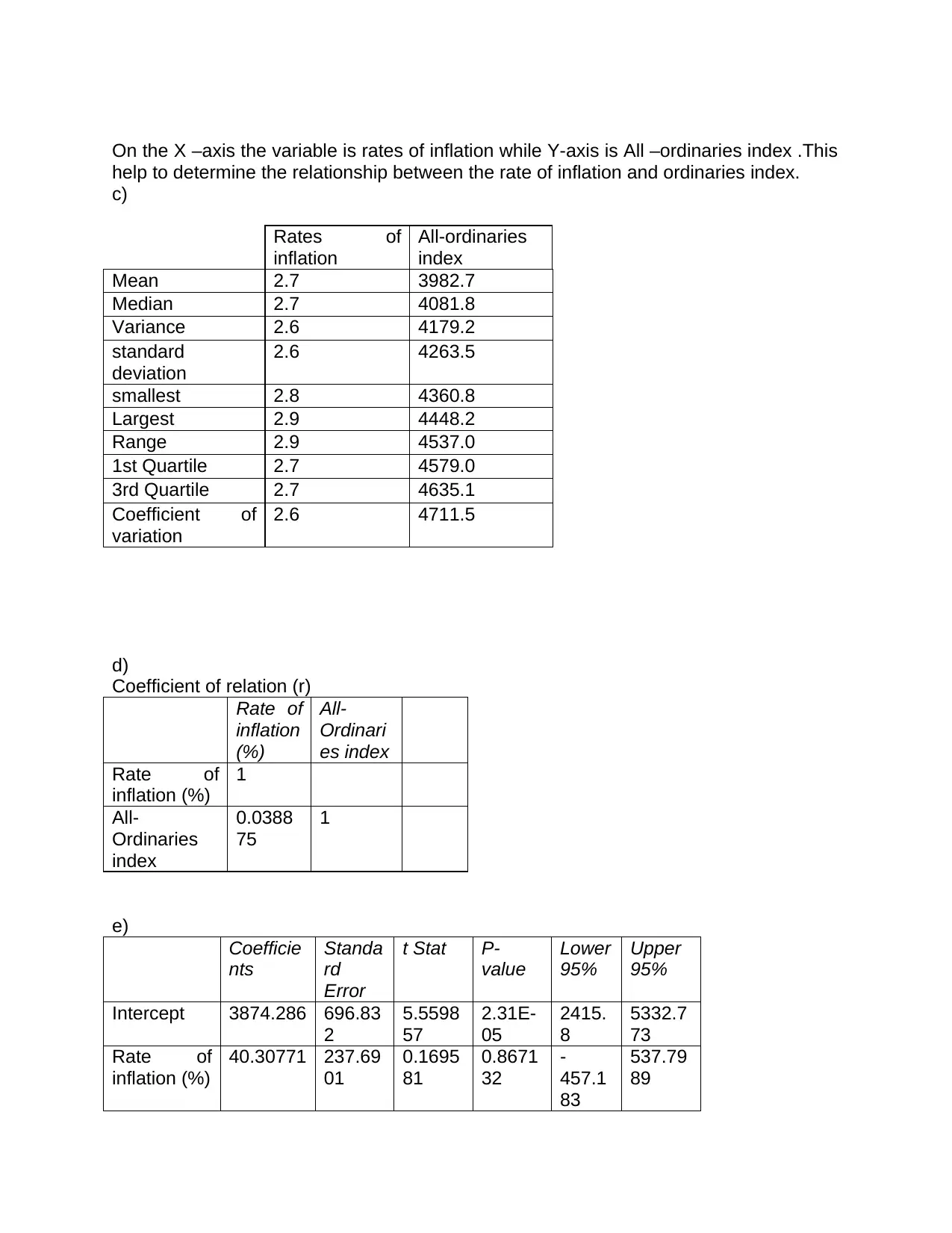
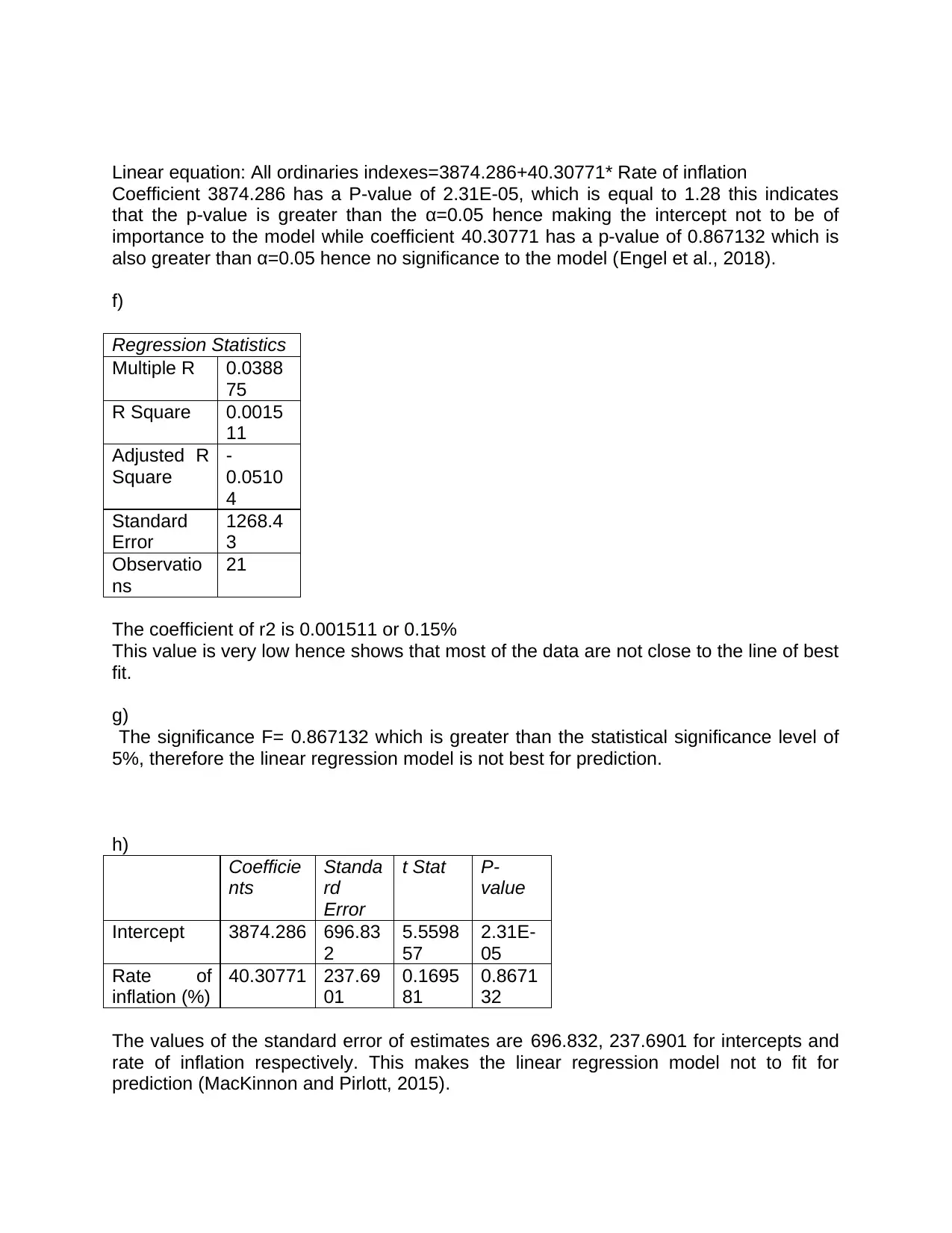
This assignment solution addresses several statistical problems related to business decision-making. Question 1 analyzes CO2 emissions from producer countries, comparing data from 2009 and 2013 using bar graphs and pie charts. Question 2 focuses on frequency distributions, cumulative frequencies, and ogive graphs, with an example of worker welding times. Question 3 delves into the Australian inflation rate, exploring its relationship with the All-ordinaries index through regression analysis, including calculating coefficients of correlation, regression statistics, and interpreting p-values. The solution includes calculations, graphical representations, and interpretations, demonstrating an understanding of statistical concepts and their application in business contexts, with references to relevant research. This assignment was completed for the HI6007 Statistics and Research Methods for Business Decision Making course.

Question 1
a)
Producer countries of CO2 emission in 2009 and 2013
In 2009, the fifteen countries co2 emission was high at 20500 metric tons while in 2013
the emission of CO2 was at25740 metric tons. In 2009 and 2013 china was the leading
country in emission of CO2 followed closely by United States and the country with the
least emission volume was Australia (Roberts, et al., 2019).
b) Total percentage of CO2 emission in 2009 and 2013
44%
56%
1 2
United States
China
Russia
Japan
India
Germany
Canada
United Kingdom
South Korea
Italy
Iran
South Africa
France
Saudi Arabia
Australia
0
2000
4000
6000
8000
10000
12000
2009
2013
Producer countries of CO2 emmitance
Amont of CO2 emitted in 2009 and
2013

The percentage of CO2 broken down by the producer countries in 2009 was 44% as
presented by the blue color on the pie chart while the maroon color represent the
percentage 56% of CO2 broken down in 2013.
c)
From the two graphical techniques that is the bar graph on Producer countries of CO2
emission in 2009 and 2013 and the pie chart on Total percentage of CO2 emission in
2009 and 2013 it is observed that both techniques shows that it is in 2013 that the
emission of CO2 was high compared to 2009.Observation made on the bar graph on
Producer countries of CO2 emission in 2009 and 2013 is that china and United states
are the leading emitting countries of CO2.
Question 2
a)
classe
s
Frequenc
y
Relative
frequency
35-44 2 0.222222222
45-54 1 0.111111111
55-64 1 0.111111111
65-74 4 0.444444444
75-84 0 0
85-94 0 0
95-
104
1 0.111111111
Total 9
b)
classes Frequenc
y
Cumulative frequency cumulative relative
frequency
35-44 2 2 0.222222222
45-54 1 3 0.333333333
55-64 1 4 0.444444444
65-74 4 8 0.888888889
75-84 0 8 0.888888889
85-94 0 8 0.888888889
95-104 1 9 1
Total 9

c)
Time required for workers at a car plant to weld cars
39.5 49.5 59.5 69.5 79.5 89.5 99.5 More
0
1
2
3
4
5
6
7
8
number of worker
Freque ncy(in tim e )
d)
Ogive graph on the number of workers and
time used.
49.5 59.5 69.5 79.5 89.5 99.5 More
0
1
2
3
4
5
6
7
0.00%
20.00%
40.00%
60.00%
80.00%
100.00%
120.00%
Frequency
Cumulative %
39.5
Frequency
e)
Proportion of the data less than 65
65-35=30
30/104 = 0.288

f)
75 more than the proportion data
104-76=28
28/104=0.269
Question 3
a)
The Australian inflation rate
1995
1997
1999
2001
2003
2005
2007
2009
2011
2013
2015
0.0
1000.0
2000.0
3000.0
4000.0
5000.0
6000.0
7000.0
Rate of inflation (%)
All-Ordinaries index
years
b)
Relationship between rate of inflation and All -ordinaries index
0.0 1.0 2.0 3.0 4.0 5.0 6.0 7.0
0.0
1000.0
2000.0
3000.0
4000.0
5000.0
6000.0
7000.0
rate of inflation
All-ordinaries index

On the X –axis the variable is rates of inflation while Y-axis is All –ordinaries index .This
help to determine the relationship between the rate of inflation and ordinaries index.
c)
Rates of
inflation
All-ordinaries
index
Mean 2.7 3982.7
Median 2.7 4081.8
Variance 2.6 4179.2
standard
deviation
2.6 4263.5
smallest 2.8 4360.8
Largest 2.9 4448.2
Range 2.9 4537.0
1st Quartile 2.7 4579.0
3rd Quartile 2.7 4635.1
Coefficient of
variation
2.6 4711.5
d)
Coefficient of relation (r)
Rate of
inflation
(%)
All-
Ordinari
es index
Rate of
inflation (%)
1
All-
Ordinaries
index
0.0388
75
1
e)
Coefficie
nts
Standa
rd
Error
t Stat P-
value
Lower
95%
Upper
95%
Intercept 3874.286 696.83
2
5.5598
57
2.31E-
05
2415.
8
5332.7
73
Rate of
inflation (%)
40.30771 237.69
01
0.1695
81
0.8671
32
-
457.1
83
537.79
89

Linear equation: All ordinaries indexes=3874.286+40.30771* Rate of inflation
Coefficient 3874.286 has a P-value of 2.31E-05, which is equal to 1.28 this indicates
that the p-value is greater than the α=0.05 hence making the intercept not to be of
importance to the model while coefficient 40.30771 has a p-value of 0.867132 which is
also greater than α=0.05 hence no significance to the model (Engel et al., 2018).
f)
Regression Statistics
Multiple R 0.0388
75
R Square 0.0015
11
Adjusted R
Square
-
0.0510
4
Standard
Error
1268.4
3
Observatio
ns
21
The coefficient of r2 is 0.001511 or 0.15%
This value is very low hence shows that most of the data are not close to the line of best
fit.
g)
The significance F= 0.867132 which is greater than the statistical significance level of
5%, therefore the linear regression model is not best for prediction.
h)
Coefficie
nts
Standa
rd
Error
t Stat P-
value
Intercept 3874.286 696.83
2
5.5598
57
2.31E-
05
Rate of
inflation (%)
40.30771 237.69
01
0.1695
81
0.8671
32
The values of the standard error of estimates are 696.832, 237.6901 for intercepts and
rate of inflation respectively. This makes the linear regression model not to fit for
prediction (MacKinnon and Pirlott, 2015).

Reference
MacKinnon, D.P. and Pirlott, A.G., 2015. Statistical approaches for enhancing causal
interpretation of the M to Y relation in mediation analysis. Personality and Social
Psychology Review, 19(1), pp.30-43.
Roberts, J.J., Leplastrier, A., Feitz, A.J., Shipton, Z.K., Bell, A.F. and Karolytė, R., 2019.
Structural controls on the location and distribution of CO2 emission at a natural CO2
spring in Daylesford, Australia. International Journal of Greenhouse Gas Control, 84,
pp.36-46.
Engel, L.C., Landmesser, U.L., Abdelwahed, Y.A., Gigengack, K.G., Manes, C.M.,
Wurster, T.H.W., Skurk, C.S., Leistner, D.L., Lauten, A.L., Schuster, A.S. and Noutsias,
M.N., 2018. P6208 Endothelial damage and its relation to coronary artery stenosis. A
correlation between molecular cardiovascular magnetic resonance imaging, and
quantitative coronary angiography. European Heart Journal, 39(suppl_1), pp.ehy566-
P6208.