HI6007 Statistics & Research Methods: Export, Sales Data Analysis

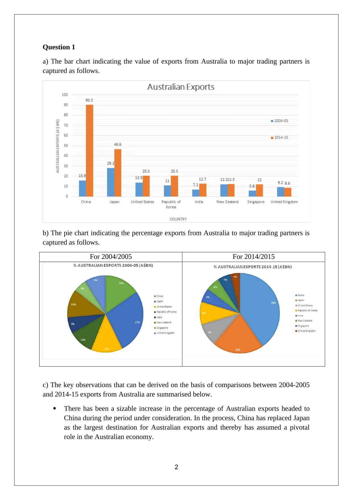
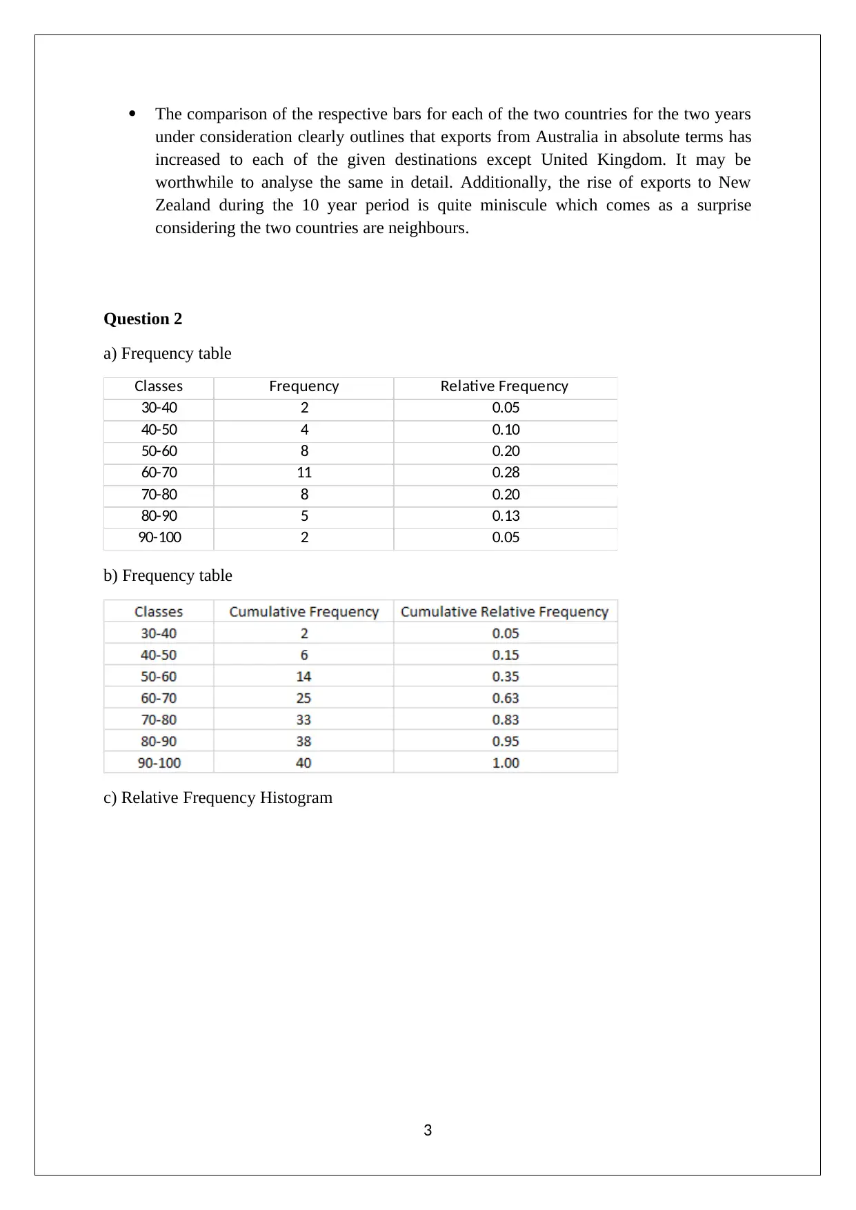
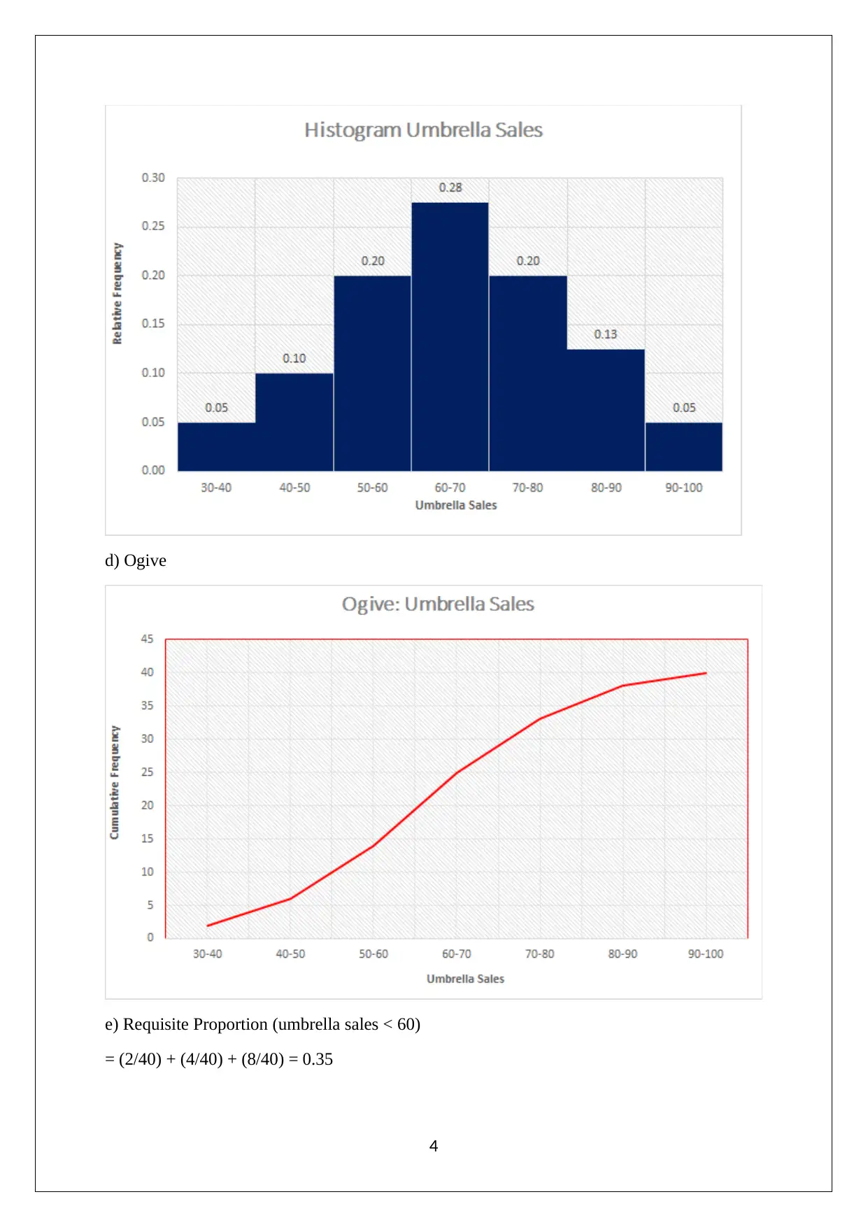
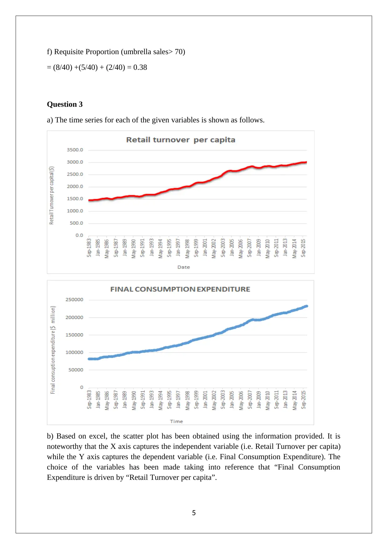
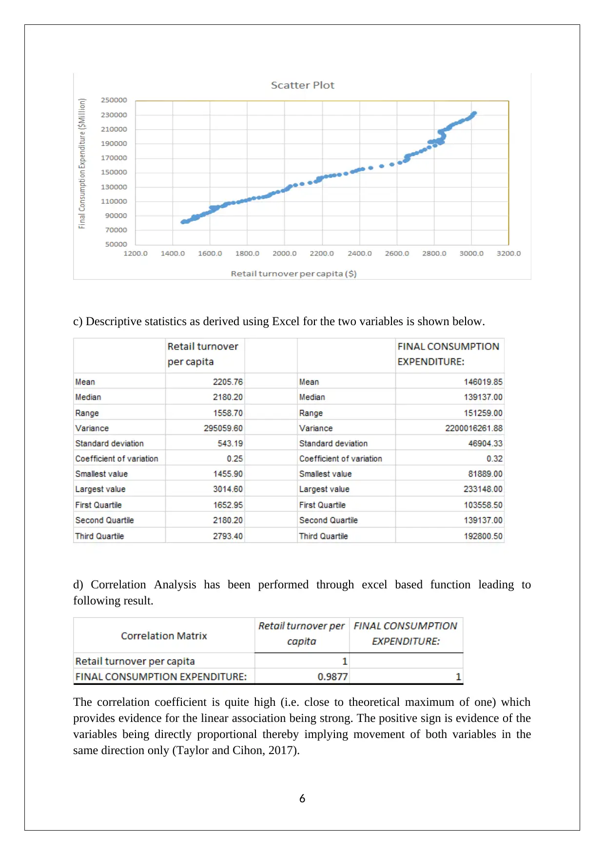
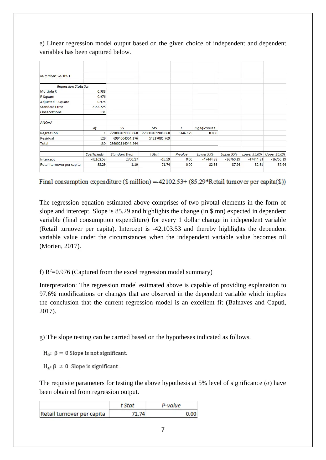
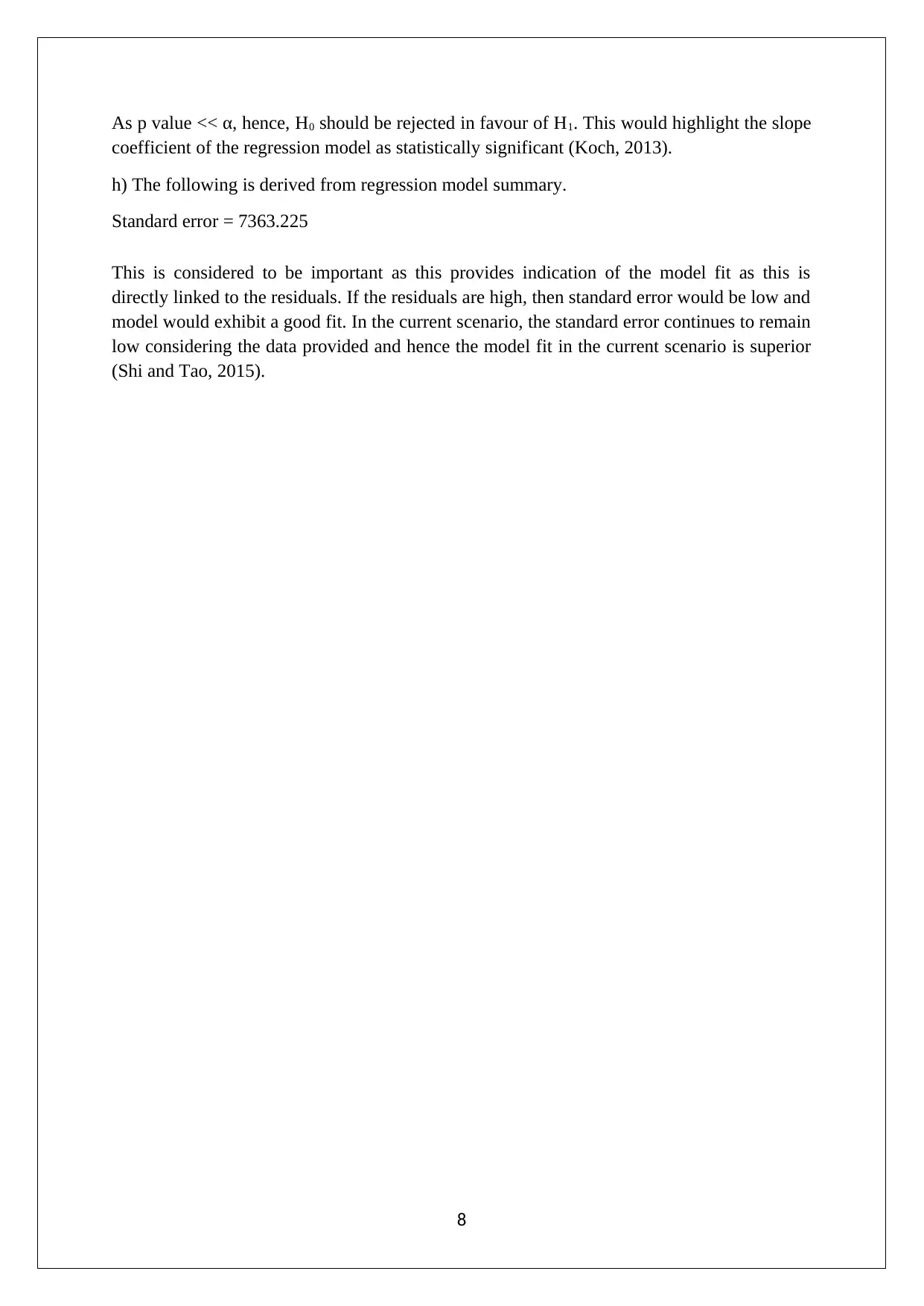
This assignment provides a detailed statistical analysis of Australian export data and retail turnover per capita. It includes bar and pie charts illustrating export values and percentages to major trading partners between 2004-2005 and 2014-2015, highlighting the significant increase in exports to China. The assignment also features frequency tables, histograms, and ogives related to umbrella sales data. Furthermore, it conducts a time series and scatter plot analysis of retail turnover per capita and final consumption expenditure, along with descriptive statistics, correlation analysis, and a linear regression model. The regression model's slope, intercept, R-squared value, and standard error are interpreted, and a hypothesis test is performed on the slope coefficient. This document is available on Desklib, a platform offering a range of study tools and solved assignments for students.

STATISTICS
STUDENT ID:
[Pick the date]

Question 1
a) The bar chart indicating the value of exports from Australia to major trading partners is
captured as follows.
b) The pie chart indicating the percentage exports from Australia to major trading partners is
captured as follows.
For 2004/2005 For 2014/2015
c) The key observations that can be derived on the basis of comparisons between 2004-2005
and 2014-15 exports from Australia are summarised below.
 There has been a sizable increase in the percentage of Australian exports headed to
China during the period under consideration. In the process, China has replaced Japan
as the largest destination for Australian exports and thereby has assumed a pivotal
role in the Australian economy.
2

 The comparison of the respective bars for each of the two countries for the two years
under consideration clearly outlines that exports from Australia in absolute terms has
increased to each of the given destinations except United Kingdom. It may be
worthwhile to analyse the same in detail. Additionally, the rise of exports to New
Zealand during the 10 year period is quite miniscule which comes as a surprise
considering the two countries are neighbours.
Question 2
a) Frequency table
Classes Frequency Relative Frequency
30-40 2 0.05
40-50 4 0.10
50-60 8 0.20
60-70 11 0.28
70-80 8 0.20
80-90 5 0.13
90-100 2 0.05
b) Frequency table
c) Relative Frequency Histogram
3

d) Ogive
e) Requisite Proportion (umbrella sales < 60)
= (2/40) + (4/40) + (8/40) = 0.35
4

f) Requisite Proportion (umbrella sales> 70)
= (8/40) +(5/40) + (2/40) = 0.38
Question 3
a) The time series for each of the given variables is shown as follows.
b) Based on excel, the scatter plot has been obtained using the information provided. It is
noteworthy that the X axis captures the independent variable (i.e. Retail Turnover per capita)
while the Y axis captures the dependent variable (i.e. Final Consumption Expenditure). The
choice of the variables has been made taking into reference that “Final Consumption
Expenditure is driven by “Retail Turnover per capita”.
5

c) Descriptive statistics as derived using Excel for the two variables is shown below.
d) Correlation Analysis has been performed through excel based function leading to
following result.
The correlation coefficient is quite high (i.e. close to theoretical maximum of one) which
provides evidence for the linear association being strong. The positive sign is evidence of the
variables being directly proportional thereby implying movement of both variables in the
same direction only (Taylor and Cihon, 2017).
6

e) Linear regression model output based on the given choice of independent and dependent
variables has been captured below.
The regression equation estimated above comprises of two pivotal elements in the form of
slope and intercept. Slope is 85.29 and highlights the change (in $ mn) expected in dependent
variable (final consumption expenditure) for every 1 dollar change in independent variable
(Retail turnover per capita). Intercept is -42,103.53 and thereby highlights the dependent
variable value under the circumstances when the independent variable value becomes nil
(Morien, 2017).
f) R2=0.976 (Captured from the excel regression model summary)
Interpretation: The regression model estimated above is capable of providing explanation to
97.6% modifications or changes that are observed in the dependent variable which implies
the conclusion that the current regression model is an excellent fit (Balnaves and Caputi,
2017).
g) The slope testing can be carried based on the hypotheses indicated as follows.
The requisite parameters for testing the above hypothesis at 5% level of significance (α) have
been obtained from regression output.
7

As p value << α, hence, H0 should be rejected in favour of H1. This would highlight the slope
coefficient of the regression model as statistically significant (Koch, 2013).
h) The following is derived from regression model summary.
Standard error = 7363.225
This is considered to be important as this provides indication of the model fit as this is
directly linked to the residuals. If the residuals are high, then standard error would be low and
model would exhibit a good fit. In the current scenario, the standard error continues to remain
low considering the data provided and hence the model fit in the current scenario is superior
(Shi and Tao, 2015).
8

References
Koch, K.R. (2013) Parameter Estimation and Hypothesis Testing in Linear Models. 2nd ed.
London: Springer Science & Business Media.
Shi, Z. N. and Tao, J. (2015) Statistical Hypothesis Testing: Theory and Methods. 6th
ed.London : World Scientific.
Taylor, K. J. and Cihon, C. (2017) Statistical Techniques for Data Analysis. 2nd ed.
Melbourne: CRC Press.
Morien, D. (2017) Business Statistics. Melbourne: Cengage learning Australia.
Balnaves, M. and Caputi, P. (2017) Introduction to Quantitative Research Methods: An
Investigation Approach. London: SAGE
9