Analyzing Stock Returns with Hypothesis Testing - Statistics
VerifiedAdded on 2023/04/03
|10
|1412
|265
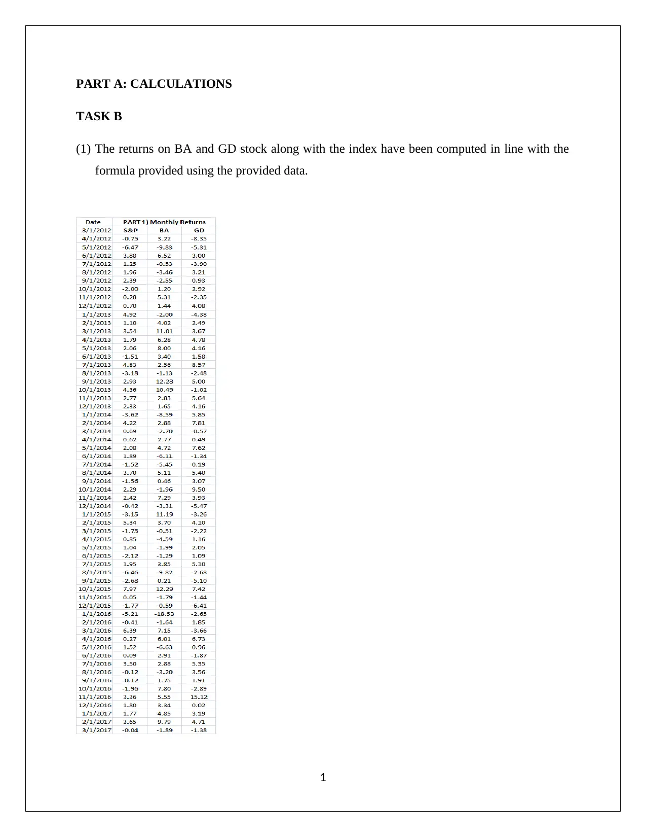
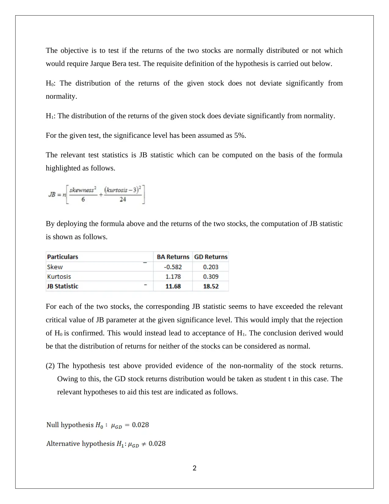
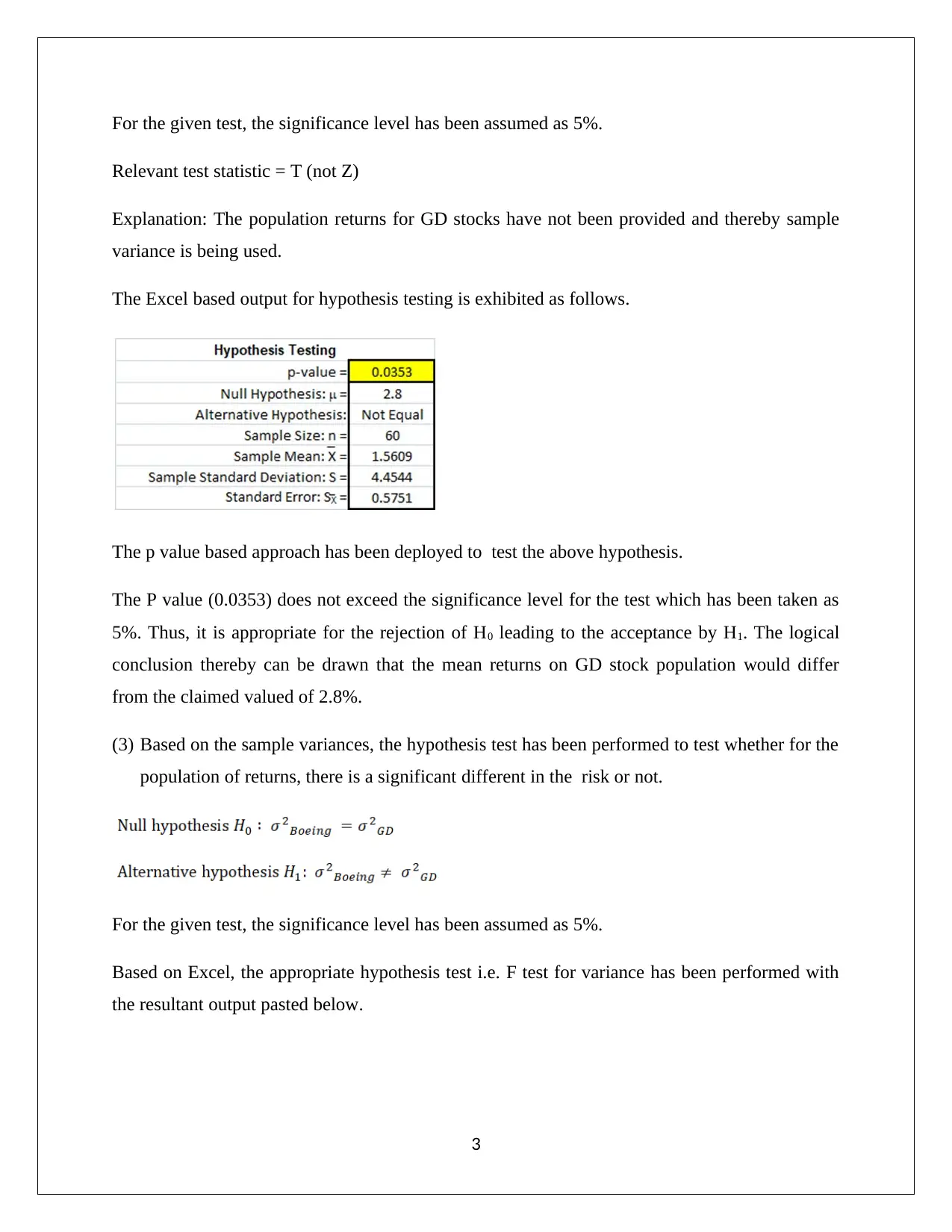
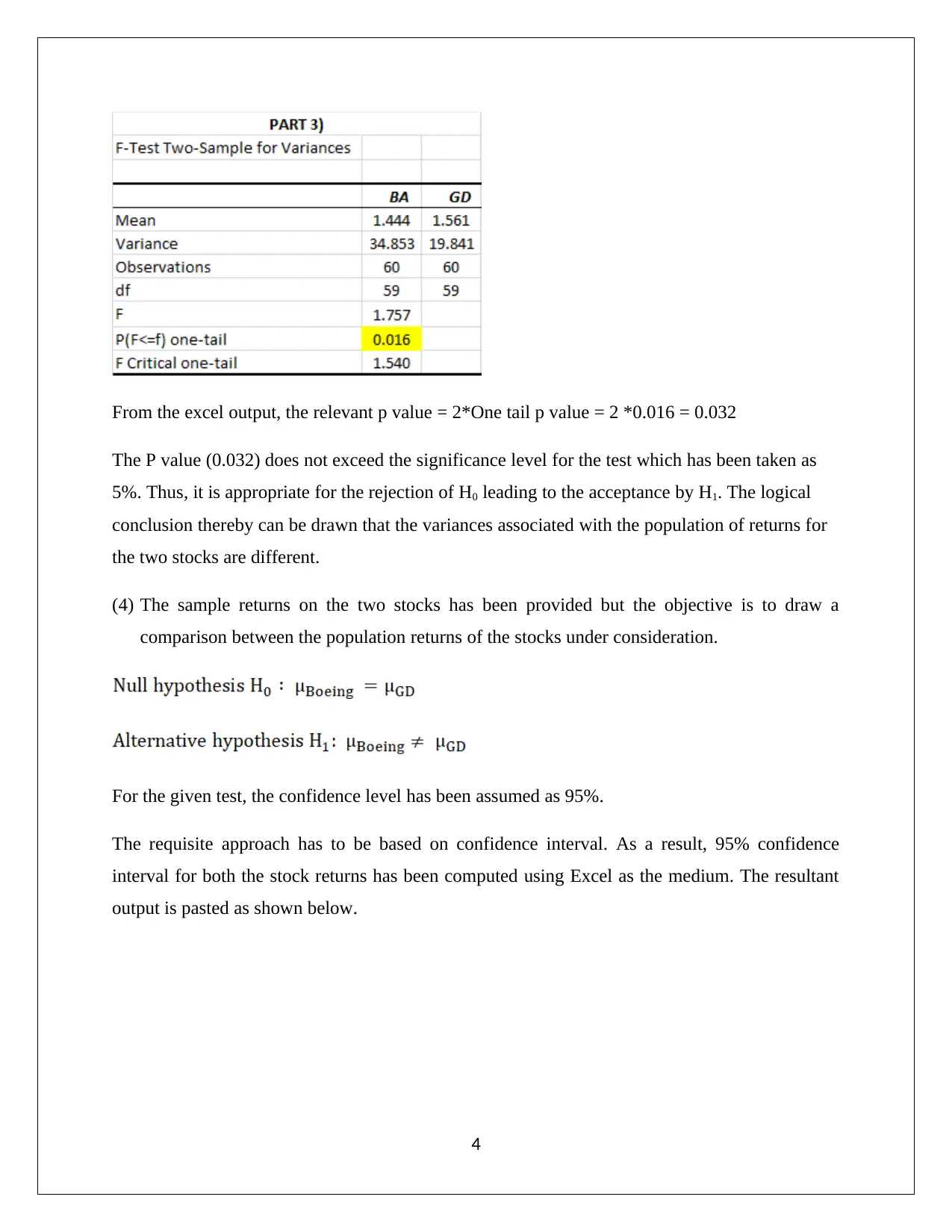
Homework Assignment
AI Summary
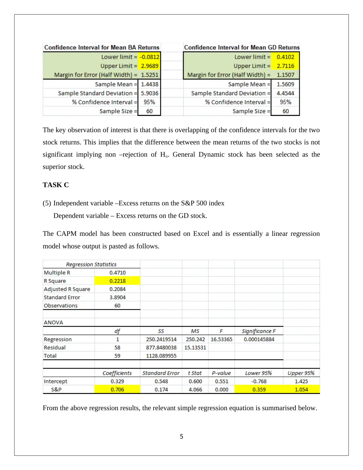
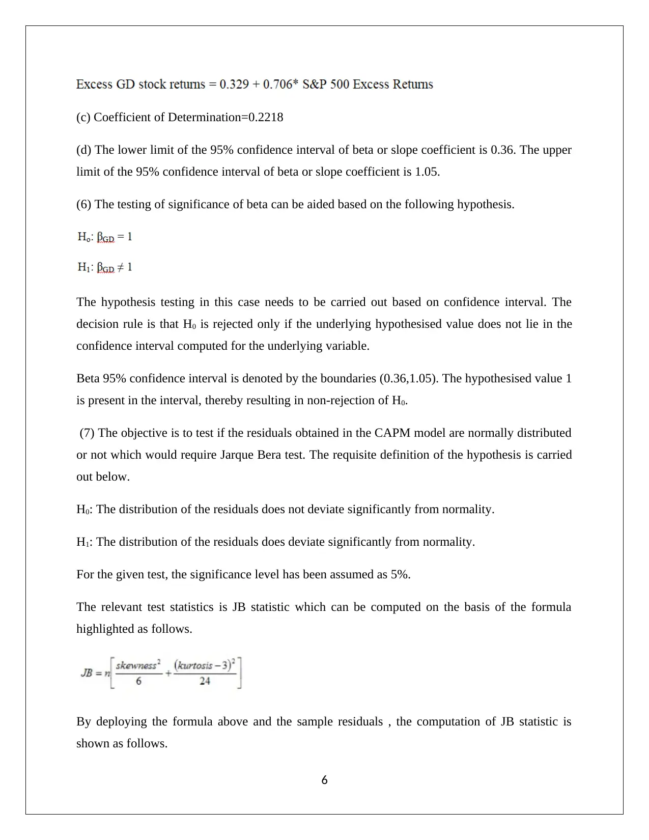
This assignment solution focuses on the statistical analysis of stock returns using hypothesis testing. It begins by testing the normality of returns for BA and GD stocks using the Jarque-Bera test, concluding that neither follows a normal distribution. Subsequently, a t-test is applied to assess if the mean returns of GD stock differ from a claimed value. An F-test is then used to determine if there's a significant difference in the risk (variance) between the two stocks. Confidence intervals are constructed to compare the population returns of the stocks. Furthermore, the assignment employs the CAPM model to analyze the relationship between excess returns on the GD stock and the S&P 500 index, including regression analysis, calculation of the coefficient of determination, and hypothesis testing for the beta coefficient. Finally, it tests the normality of residuals from the CAPM model. Desklib offers a wide array of similar solved assignments and study resources for students.


1 out of 10
Related Documents


![Statistical Analysis of Business and Finance Data - [Semester]](/_next/image/?url=https%3A%2F%2Fdesklib.com%2Fmedia%2Fbusiness-finance-statistics-hypothesis-interpretation_page_2.jpg&w=256&q=75)

Your All-in-One AI-Powered Toolkit for Academic Success.
+13062052269
info@desklib.com
Available 24*7 on WhatsApp / Email
![[object Object]](/_next/static/media/star-bottom.7253800d.svg)
Copyright © 2020–2026 A2Z Services. All Rights Reserved. Developed and managed by ZUCOL.