Decision Support Tool Analysis and Statistics Assignment Solution

This document presents a complete solution to a statistics assignment centered on a decision support tool. It begins by defining random variables and differentiating between discrete and continuous types, including the concept of expected value and its calculation. The assignment then delves into probability calculations, including determining the probability of sales within certain ranges and applying the normal distribution to assess sales probabilities. The document proceeds to analyze demographic data, calculating probabilities based on age and sex. Finally, it addresses statistical process control, calculating control limits and confidence intervals for labor hours, and concludes with a hypothesis test to evaluate the impact of occupational safety training on sick days. The solution incorporates relevant statistical formulas and interpretations throughout.

Running Head: DECISION SUPPORT TOOL
Decision Support Tool
Name of the Student
Name of the University
Author Note

1DECISION SUPPORT TOOL
Table of Contents
ANSWER 1.....................................................................................................................................2
ANSWER 2.....................................................................................................................................5
ANSWER 3.....................................................................................................................................6
REFERENCES................................................................................................................................8

2DECISION SUPPORT TOOL
ANSWER 1
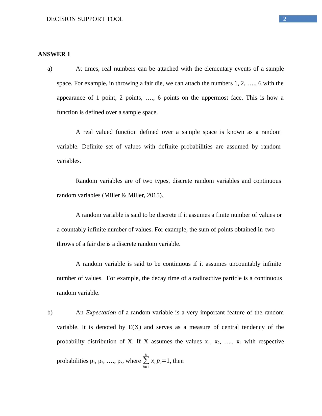
a) At times, real numbers can be attached with the elementary events of a sample
space. For example, in throwing a fair die, we can attach the numbers 1, 2, …., 6 with the
appearance of 1 point, 2 points, …., 6 points on the uppermost face. This is how a
function is defined over a sample space.
A real valued function defined over a sample space is known as a random
variable. Definite set of values with definite probabilities are assumed by random
variables.
Random variables are of two types, discrete random variables and continuous
random variables (Miller & Miller, 2015).
A random variable is said to be discrete if it assumes a finite number of values or
a countably infinite number of values. For example, the sum of points obtained in two
throws of a fair die is a discrete random variable.
A random variable is said to be continuous if it assumes uncountably infinite
number of values. For example, the decay time of a radioactive particle is a continuous
random variable.
b) An Expectation of a random variable is a very important feature of the random
variable. It is denoted by E(X) and serves as a measure of central tendency of the
probability distribution of X. If X assumes the values x1, x2, …., xk with respective
probabilities p1, p2, …., pk, where ∑
i=1
k
xi pi=1, then

3DECISION SUPPORT TOOL
E ( X ) =∑
i=1
k
xi pi, provided it is finite.
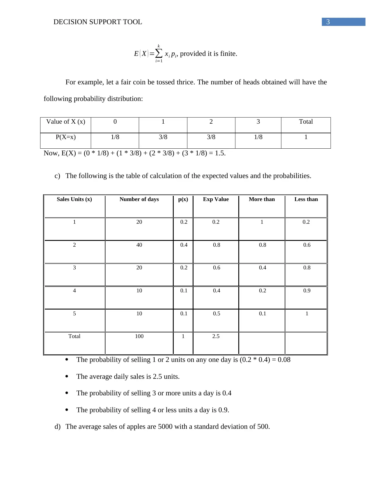
For example, let a fair coin be tossed thrice. The number of heads obtained will have the
following probability distribution:
Value of X (x) 0 1 2 3 Total
P(X=x) 1/8 3/8 3/8 1/8 1
Now, E(X) = (0 * 1/8) + (1 * 3/8) + (2 * 3/8) + (3 * 1/8) = 1.5.
c) The following is the table of calculation of the expected values and the probabilities.
Sales Units (x) Number of days p(x) Exp Value More than Less than
1 20 0.2 0.2 1 0.2
2 40 0.4 0.8 0.8 0.6
3 20 0.2 0.6 0.4 0.8
4 10 0.1 0.4 0.2 0.9
5 10 0.1 0.5 0.1 1
Total 100 1 2.5
 The probability of selling 1 or 2 units on any one day is (0.2 * 0.4) = 0.08
 The average daily sales is 2.5 units.
 The probability of selling 3 or more units a day is 0.4
 The probability of selling 4 or less units a day is 0.9.
d) The average sales of apples are 5000 with a standard deviation of 500.

4DECISION SUPPORT TOOL
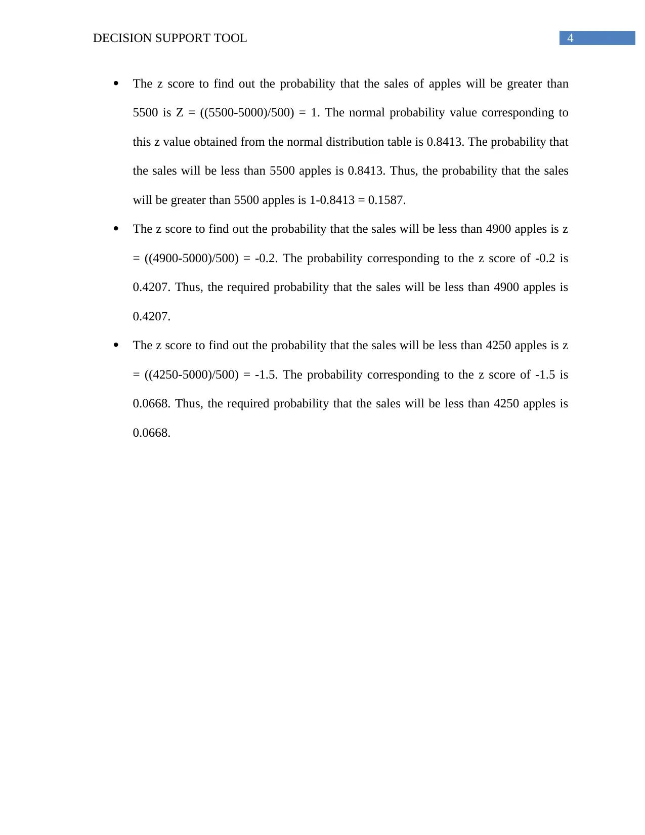
 The z score to find out the probability that the sales of apples will be greater than
5500 is Z = ((5500-5000)/500) = 1. The normal probability value corresponding to
this z value obtained from the normal distribution table is 0.8413. The probability that
the sales will be less than 5500 apples is 0.8413. Thus, the probability that the sales
will be greater than 5500 apples is 1-0.8413 = 0.1587.
 The z score to find out the probability that the sales will be less than 4900 apples is z
= ((4900-5000)/500) = -0.2. The probability corresponding to the z score of -0.2 is
0.4207. Thus, the required probability that the sales will be less than 4900 apples is
0.4207.
 The z score to find out the probability that the sales will be less than 4250 apples is z
= ((4250-5000)/500) = -1.5. The probability corresponding to the z score of -1.5 is
0.0668. Thus, the required probability that the sales will be less than 4250 apples is
0.0668.

5DECISION SUPPORT TOOL
ANSWER 2
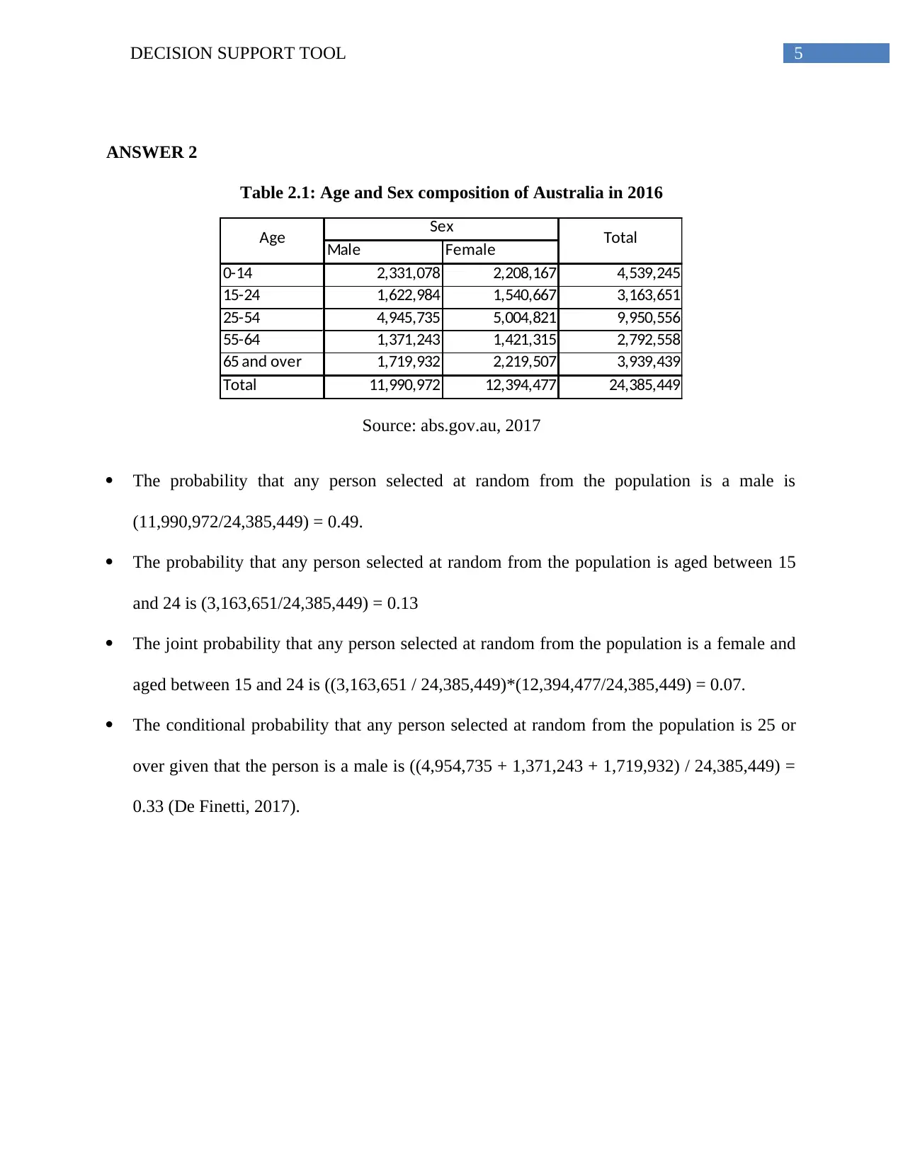
Table 2.1: Age and Sex composition of Australia in 2016
Male Female
0-14 2,331,078 2,208,167 4,539,245
15-24 1,622,984 1,540,667 3,163,651
25-54 4,945,735 5,004,821 9,950,556
55-64 1,371,243 1,421,315 2,792,558
65 and over 1,719,932 2,219,507 3,939,439
Total 11,990,972 12,394,477 24,385,449
Age Sex Total
Source: abs.gov.au, 2017
 The probability that any person selected at random from the population is a male is
(11,990,972/24,385,449) = 0.49.
 The probability that any person selected at random from the population is aged between 15
and 24 is (3,163,651/24,385,449) = 0.13
 The joint probability that any person selected at random from the population is a female and
aged between 15 and 24 is ((3,163,651 / 24,385,449)*(12,394,477/24,385,449) = 0.07.
 The conditional probability that any person selected at random from the population is 25 or
over given that the person is a male is ((4,954,735 + 1,371,243 + 1,719,932) / 24,385,449) =
0.33 (De Finetti, 2017).

6DECISION SUPPORT TOOL
ANSWER 3
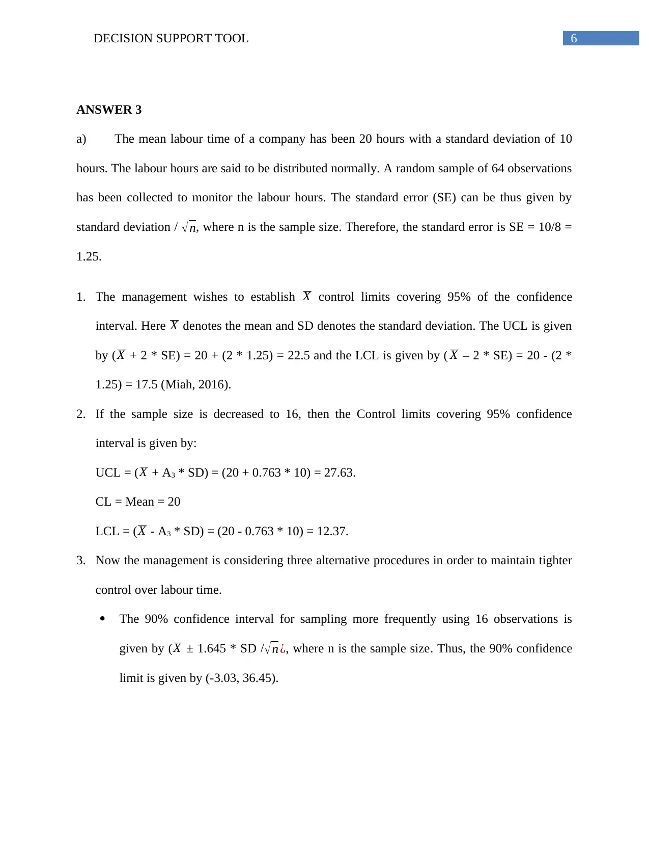
a) The mean labour time of a company has been 20 hours with a standard deviation of 10
hours. The labour hours are said to be distributed normally. A random sample of 64 observations
has been collected to monitor the labour hours. The standard error (SE) can be thus given by
standard deviation / √n, where n is the sample size. Therefore, the standard error is SE = 10/8 =
1.25.
1. The management wishes to establish X control limits covering 95% of the confidence
interval. Here X denotes the mean and SD denotes the standard deviation. The UCL is given
by (X + 2 * SE) = 20 + (2 * 1.25) = 22.5 and the LCL is given by ( X – 2 * SE) = 20 - (2 *
1.25) = 17.5 (Miah, 2016).
2. If the sample size is decreased to 16, then the Control limits covering 95% confidence
interval is given by:
UCL = (X + A3 * SD) = (20 + 0.763 * 10) = 27.63.
CL = Mean = 20
LCL = (X - A3 * SD) = (20 - 0.763 * 10) = 12.37.
3. Now the management is considering three alternative procedures in order to maintain tighter
control over labour time.
 The 90% confidence interval for sampling more frequently using 16 observations is
given by ( X ± 1.645 * SD / √n ¿, where n is the sample size. Thus, the 90% confidence
limit is given by (-3.03, 36.45).

7DECISION SUPPORT TOOL
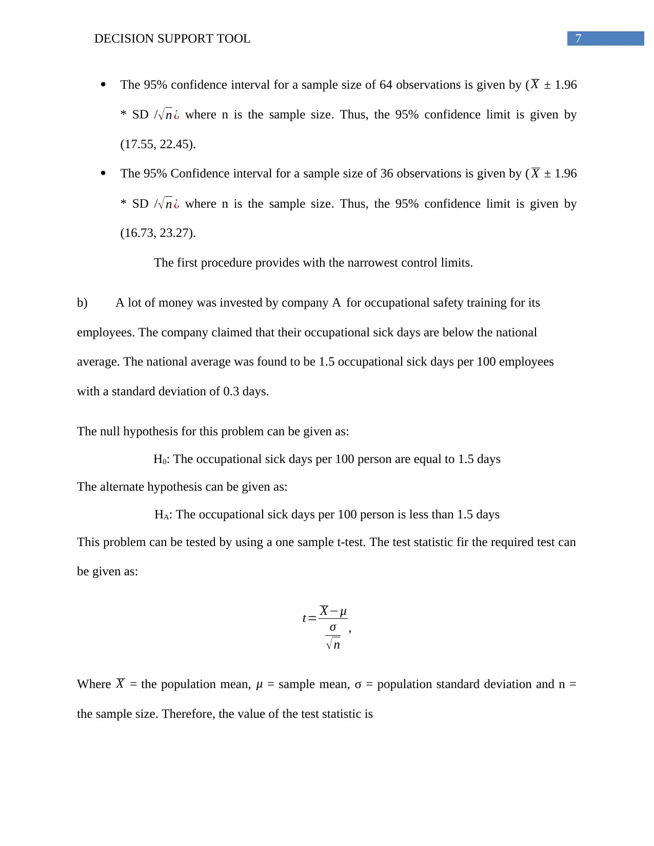
 The 95% confidence interval for a sample size of 64 observations is given by ( X ± 1.96
* SD / √n ¿ where n is the sample size. Thus, the 95% confidence limit is given by
(17.55, 22.45).
 The 95% Confidence interval for a sample size of 36 observations is given by ( X ± 1.96
* SD / √n ¿ where n is the sample size. Thus, the 95% confidence limit is given by
(16.73, 23.27).
The first procedure provides with the narrowest control limits.
b) A lot of money was invested by company A for occupational safety training for its
employees. The company claimed that their occupational sick days are below the national
average. The national average was found to be 1.5 occupational sick days per 100 employees
with a standard deviation of 0.3 days.
The null hypothesis for this problem can be given as:
H0: The occupational sick days per 100 person are equal to 1.5 days
The alternate hypothesis can be given as:
HA: The occupational sick days per 100 person is less than 1.5 days
This problem can be tested by using a one sample t-test. The test statistic fir the required test can
be given as:
t= X−μ
σ
√ n
,
Where X = the population mean, μ = sample mean, σ = population standard deviation and n =
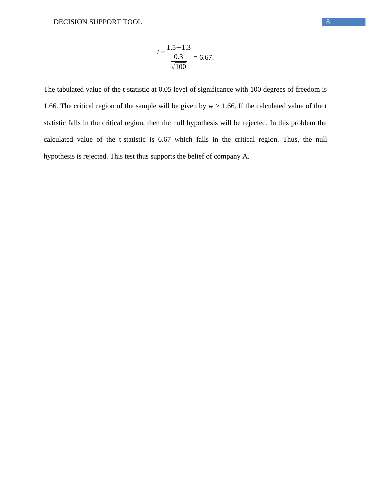
the sample size. Therefore, the value of the test statistic is

8DECISION SUPPORT TOOL
t= 1.5−1.3
0.3
√ 100
= 6.67.
The tabulated value of the t statistic at 0.05 level of significance with 100 degrees of freedom is
1.66. The critical region of the sample will be given by w > 1.66. If the calculated value of the t
statistic falls in the critical region, then the null hypothesis will be rejected. In this problem the
calculated value of the t-statistic is 6.67 which falls in the critical region. Thus, the null
hypothesis is rejected. This test thus supports the belief of company A.

9DECISION SUPPORT TOOL
REFERENCES
3101.0 - Australian Demographic Statistics, Sep 2016. (2017). Abs.gov.au. Retrieved 9 August
2017, from http://www.abs.gov.au/AUSSTATS/abs@.nsf/DetailsPage/3101.0Sep
%202016?OpenDocument
De Finetti, B. (2017). Theory of probability: A critical introductory treatment(Vol. 6). John
Wiley & Sons.
Miah, A. Q. (2016). Statistical Quality Control. In Applied Statistics for Social and Management
Sciences (pp. 353-384). Springer Singapore.
Miller, I., & Miller, M. (2015). John E. Freund's mathematical statistics with applications.
Pearson.