Statistics for Management: Annual Earnings and Economic Analysis

This report provides a comprehensive statistical analysis for management, focusing on UK earnings data from 2010 to 2016. It examines annual earnings in both public and private sectors, comparing male and female salaries, and highlighting percentage changes over the years. The report includes interpretations of gross annual earnings by industry, specifically finance and education, and administrative and healthcare staff. It further analyzes hourly payments across different UK regions, calculating mean, median, and standard deviation. Additionally, the report explores the analysis of yearly deliveries by suppliers, determining economic order quantity and suggesting a total variable cost model. Finally, it presents graphical representations, including line and Ogive charts, to illustrate gross earnings trends and cumulative sales percentages, respectively. The report utilizes various statistical techniques to provide valuable insights for management decision-making.

STATISTICS FOR
MANAGEMENT

TABLE OF CONTENTS
INTRODUCTION...........................................................................................................................1
ACTIVITY 1....................................................................................................................................1
1.1 Information with context of annual earning..........................................................................1
1.1 (A) Gross annual earning of public sector and private sector...............................................1
1.1 (B) Differences between annual earnings of male employees and female employees.........3
1.2 Interpretation of gross annual earning on National statistics website by industry................5
1.2 (A) Determining the differences in Finance and education .................................................5
1.2 (B) Analysis of Administrative staff and health and social care staff...................................7
.....................................................................................................................................................7
Activity 2.........................................................................................................................................7
2.1 Hourly Payment with respect to different regions in UK.....................................................7
2.1 (A) Estimating median..........................................................................................................7
2.1 (B) Comparing the earnings of both region..........................................................................9
Activity 3.......................................................................................................................................10
3.1 Analysis of yearly deliveries made by suppliers.................................................................10
3.2 Quantity of bags which are delivered in each period..........................................................10
3.3 Determining the Economic Order Quantity........................................................................11
3.4 Suggestion for total variable cost model.............................................................................12
Activity 4.......................................................................................................................................13
4.1 Framing a line chart which determines the gross earnings of female and male employees
during the year 2010 to 2016....................................................................................................13
4.2 Framing an Ogive chart which helps in determining the cumulative percentage of sales..15
CONCLUSION..............................................................................................................................15
REFERENCES..............................................................................................................................17

INTRODUCTION
Each and every management has the need of statistics as with the means of statistics only
financial performance of the organisation can be determined. The present report is giving brief
description about how to identify the data set and to come at the results which are favourable on
which the organisation can imply several measuring techniques. These techniques are usually
used for financial, statistical and accounting tools. While, implying these techniques it will be
giving a perfect analysis of the framework which is operational. The present report will be
identifying several figures and facts which consists of statistical data. The data set has been
analysed and along with this, detailed yearly wages of male workers and female workers in the
job of public and private sector. There is presence of various measurement of the economic order
quantity and techniques which will be pertaining the reorder level of the entity. The statistical
techniques of mean, median and standard deviation will be representing the perfect results to
every researcher on which specific decisions and alterations are taken in activities related to
operation.
ACTIVITY 1
1.1 Information with context of annual earning
1.1 (A) Gross annual earning of public sector and private sector
Gross annual salaries from the year 2010 to 2016 of public and private sector give
positive changes (Sebastianelli and Tamimi, 2011). The wages which are gained by male and
female employees of public and private sector are depicting drastic changes in these seven years.
Below table is the clear presentation:
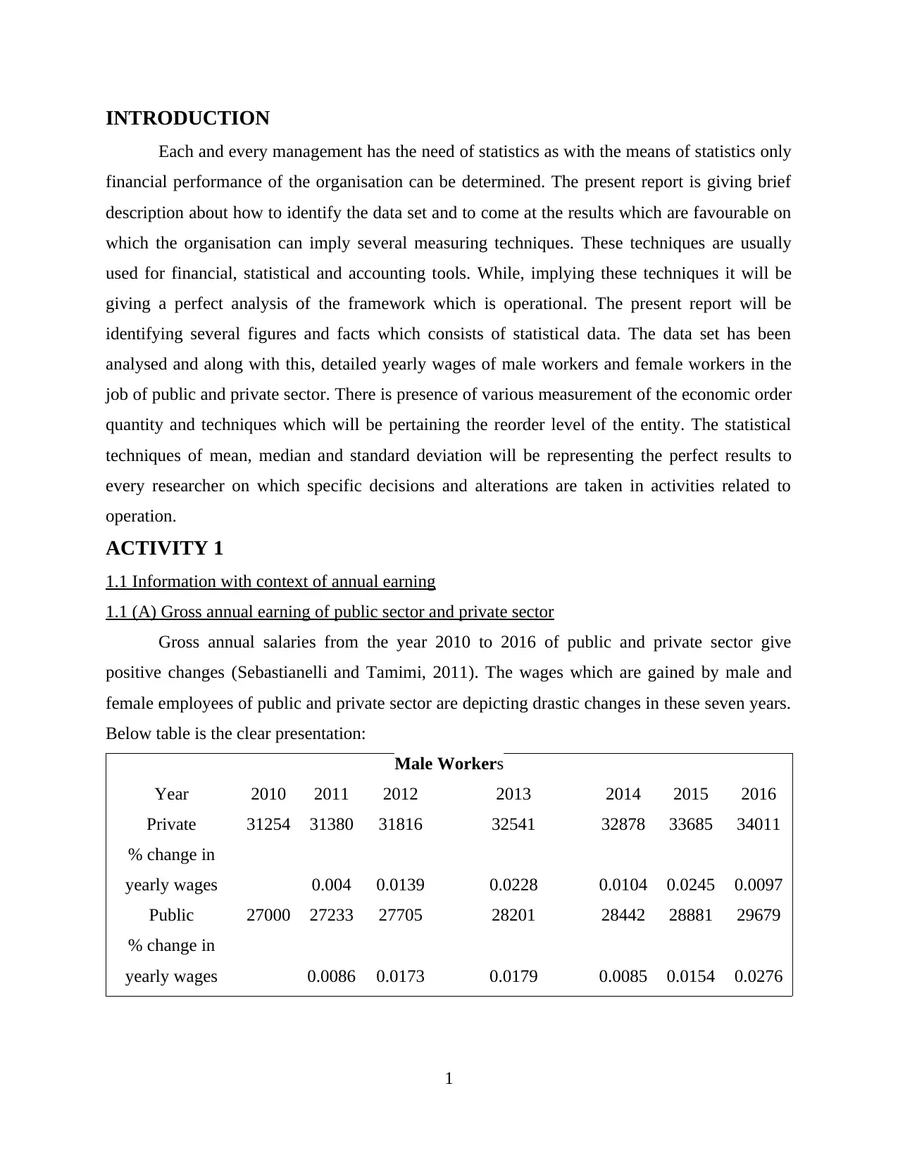
Male Workers
Year 2010 2011 2012 2013 2014 2015 2016
Private 31254 31380 31816 32541 32878 33685 34011
% change in
yearly wages 0.004 0.0139 0.0228 0.0104 0.0245 0.0097
Public 27000 27233 27705 28201 28442 28881 29679
% change in
yearly wages 0.0086 0.0173 0.0179 0.0085 0.0154 0.0276
1

2010 2011 2012 2013 2014 2015 2016
0
5000
10000
15000
20000
25000
30000
35000
Interpretation: The above graph is showing clear picture of differences in the wages of
male workers in the year 2010 to 2016 (Turkyilmaz, and et.al, 2011). The variations of male
workers of public sector and their salaries are higher than that of private sector. This graph is
presenting role of self and private employment which will lead to generate wealth of the people.
With the perspective of yearly wages with the percentage change of workers of public and
private sector, the percentage are as follows of public sector in the year of 2011 was 0.86%, 2012
is 1.73%, 2013 is 1.79%, 2014 is 1.04%, 2015 is 1.54% and in the year 2016 it is 2.76%. The
percentage changes related to private sector in the year 2011, 2012
2013, 2014, 2015 and 2016 is 0.40%, 1.39%, 2.28%, 1.04%, 2.45% and 0.97% respectively.
While observing these variations, it has been analysed that earning capacity related to male
employees has various fluctuations in the yearly earnings.
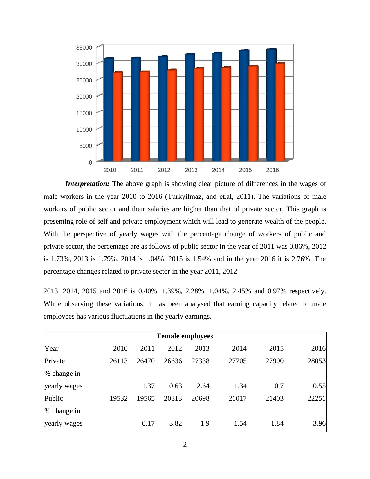
Female employees
Year 2010 2011 2012 2013 2014 2015 2016
Private 26113 26470 26636 27338 27705 27900 28053
% change in
yearly wages 1.37 0.63 2.64 1.34 0.7 0.55
Public 19532 19565 20313 20698 21017 21403 22251
% change in
yearly wages 0.17 3.82 1.9 1.54 1.84 3.96
2

Interpretation: The above graph and table is giving brief understanding on number of
female workers who are working in private and public sector as well as changes of annual
salaries with percentage change as well. The above table is presenting a clear analysis of change
in annual wages and percentage from year 2011 to 2016. The percentage change in annual wages
of female in private sector in 2011, 2012, 2013, 2014, 2014 and 2016 is 1.37%, 0.63%, 2.64%,
1.34%, 0.70% and 0.55% respectively (Lee, 2012). On the contrary, the percentage change of
female employees in context of public sector in 2011, 2012, 2013, 2014, 2015 and 2016 is
0.17%, 3.82%, 1.90%, 1.54%, 1.84% and 3.96% respectively. The above analysis is clearly
depicting that female workers of private sector are higher than public sector and with the context
of annual wages public sector is increasing.
1.1 (B) Differences between annual earnings of male employees and female employees
Private Sector
Year 2010 2011 2012 2013 2014 2015 2016
Male
Workers 31254 31380 31816 32541 32878 33685 34011
Female
Workers 26113 26470 26636 27338 27705 27900 28053
3

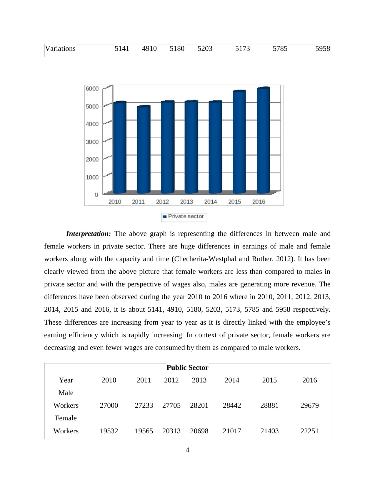
Variations 5141 4910 5180 5203 5173 5785 5958
Interpretation: The above graph is representing the differences in between male and
female workers in private sector. There are huge differences in earnings of male and female
workers along with the capacity and time (Checherita-Westphal and Rother, 2012). It has been
clearly viewed from the above picture that female workers are less than compared to males in
private sector and with the perspective of wages also, males are generating more revenue. The
differences have been observed during the year 2010 to 2016 where in 2010, 2011, 2012, 2013,
2014, 2015 and 2016, it is about 5141, 4910, 5180, 5203, 5173, 5785 and 5958 respectively.
These differences are increasing from year to year as it is directly linked with the employee’s
earning efficiency which is rapidly increasing. In context of private sector, female workers are
decreasing and even fewer wages are consumed by them as compared to male workers.
Public Sector
Year 2010 2011 2012 2013 2014 2015 2016
Male
Workers 27000 27233 27705 28201 28442 28881 29679
Female
Workers 19532 19565 20313 20698 21017 21403 22251
4

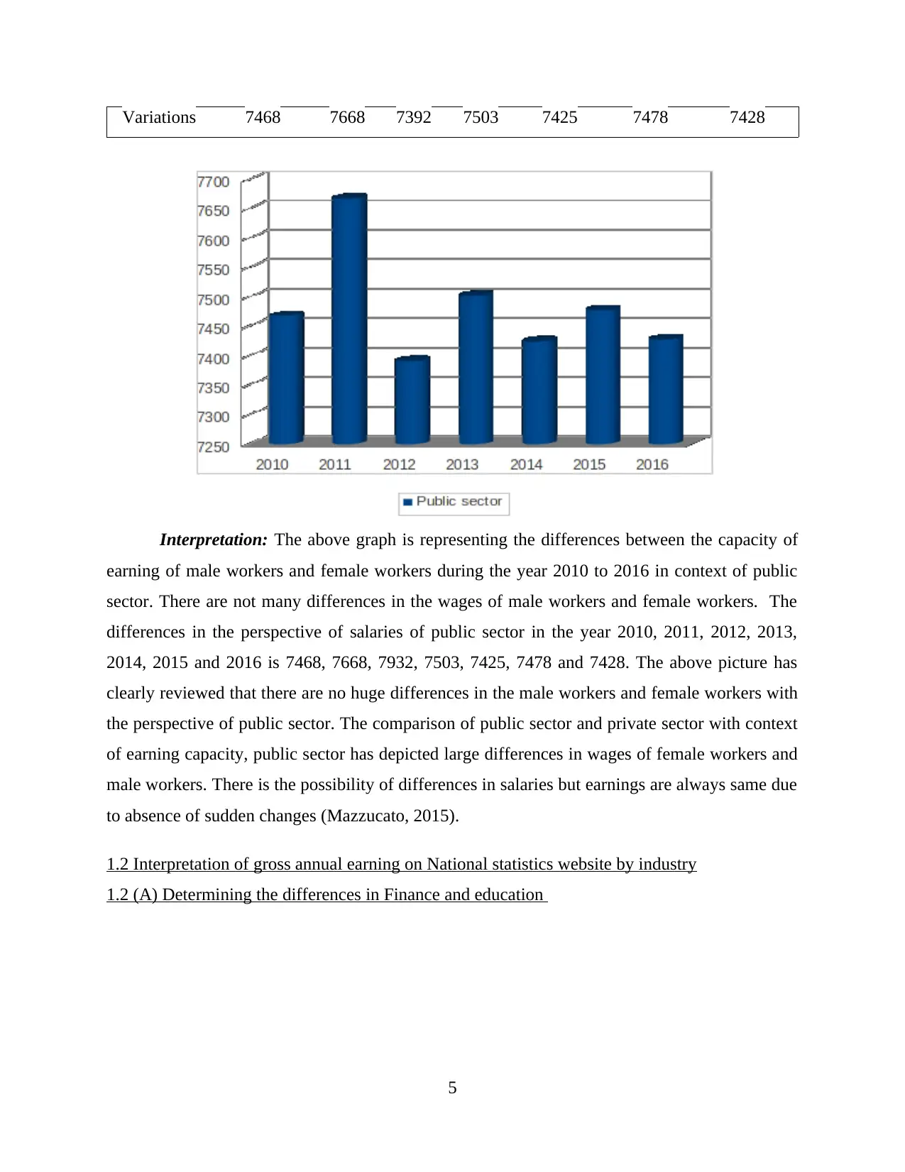
Variations 7468 7668 7392 7503 7425 7478 7428
Interpretation: The above graph is representing the differences between the capacity of
earning of male workers and female workers during the year 2010 to 2016 in context of public
sector. There are not many differences in the wages of male workers and female workers. The
differences in the perspective of salaries of public sector in the year 2010, 2011, 2012, 2013,
2014, 2015 and 2016 is 7468, 7668, 7932, 7503, 7425, 7478 and 7428. The above picture has
clearly reviewed that there are no huge differences in the male workers and female workers with
the perspective of public sector. The comparison of public sector and private sector with context
of earning capacity, public sector has depicted large differences in wages of female workers and
male workers. There is the possibility of differences in salaries but earnings are always same due
to absence of sudden changes (Mazzucato, 2015).
1.2 Interpretation of gross annual earning on National statistics website by industry
1.2 (A) Determining the differences in Finance and education
5

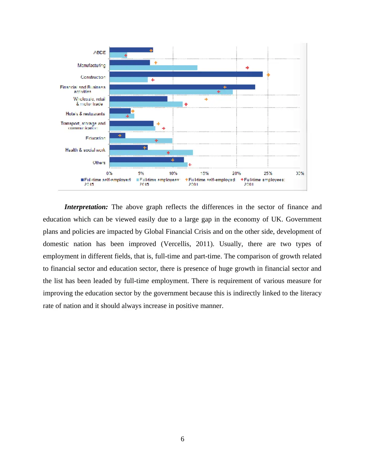
Interpretation: The above graph reflects the differences in the sector of finance and
education which can be viewed easily due to a large gap in the economy of UK. Government
plans and policies are impacted by Global Financial Crisis and on the other side, development of
domestic nation has been improved (Vercellis, 2011). Usually, there are two types of
employment in different fields, that is, full-time and part-time. The comparison of growth related
to financial sector and education sector, there is presence of huge growth in financial sector and
the list has been leaded by full-time employment. There is requirement of various measure for
improving the education sector by the government because this is indirectly linked to the literacy
rate of nation and it should always increase in positive manner.
6

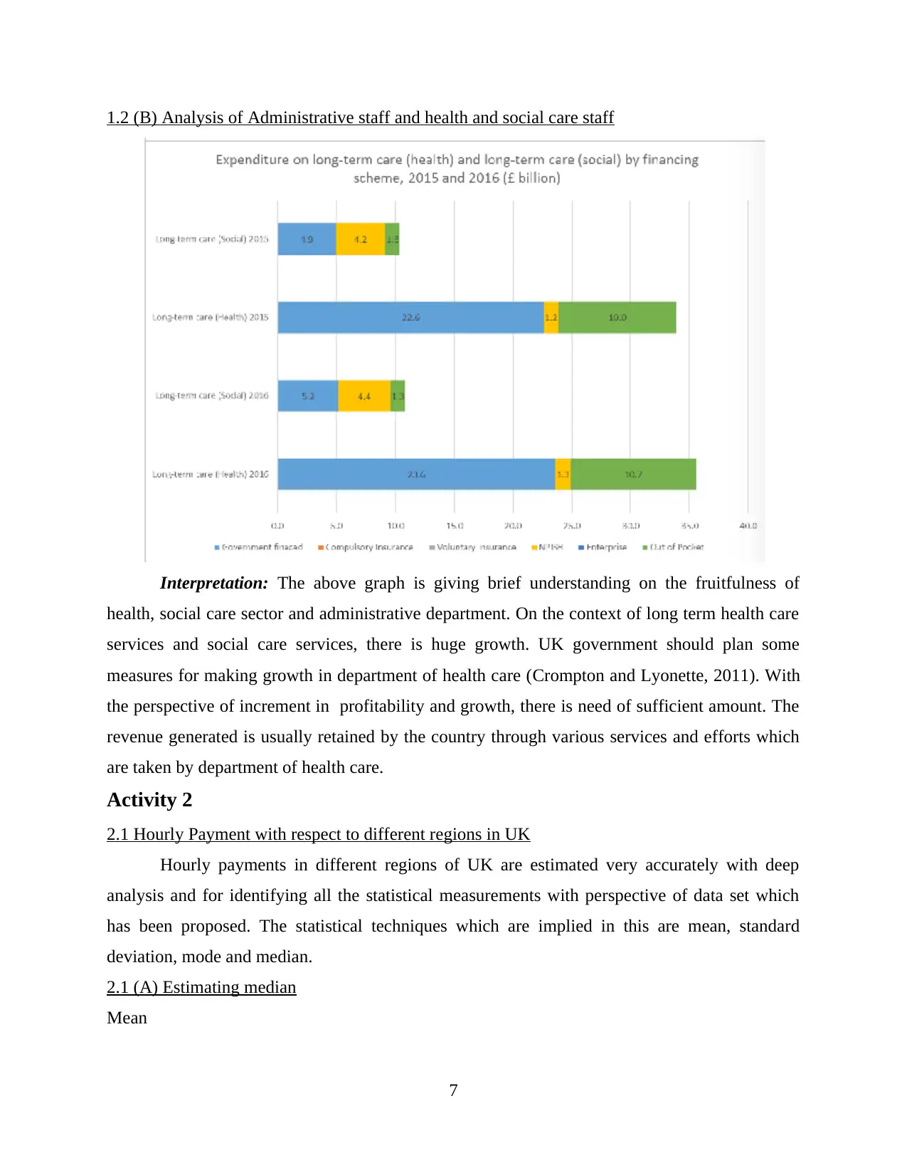
1.2 (B) Analysis of Administrative staff and health and social care staff
Interpretation: The above graph is giving brief understanding on the fruitfulness of
health, social care sector and administrative department. On the context of long term health care
services and social care services, there is huge growth. UK government should plan some
measures for making growth in department of health care (Crompton and Lyonette, 2011). With
the perspective of increment in profitability and growth, there is need of sufficient amount. The
revenue generated is usually retained by the country through various services and efforts which
are taken by department of health care.
Activity 2
2.1 Hourly Payment with respect to different regions in UK
Hourly payments in different regions of UK are estimated very accurately with deep
analysis and for identifying all the statistical measurements with perspective of data set which
has been proposed. The statistical techniques which are implied in this are mean, standard
deviation, mode and median.
2.1 (A) Estimating median
Mean
7

Salaries (hourly) Workers (%) Middle value FX
0-10 8 5 40
10 – 20 46 15 690
20-30 26 25 650
30-40 14 35 490
40-50 6 45 270
Aggregate 100 2140
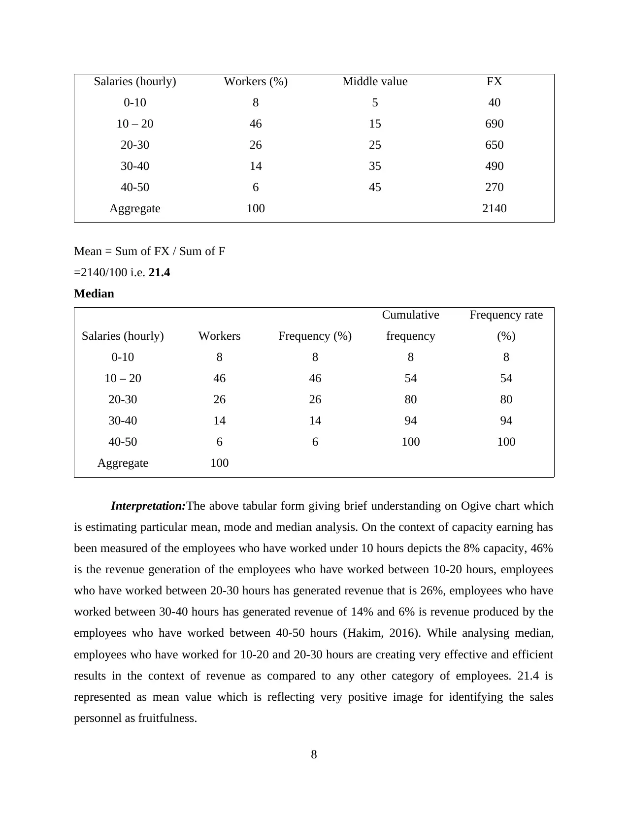
Mean = Sum of FX / Sum of F
=2140/100 i.e. 21.4
Median
Salaries (hourly) Workers Frequency (%)
Cumulative
frequency
Frequency rate
(%)
0-10 8 8 8 8
10 – 20 46 46 54 54
20-30 26 26 80 80
30-40 14 14 94 94
40-50 6 6 100 100
Aggregate 100
Interpretation:The above tabular form giving brief understanding on Ogive chart which
is estimating particular mean, mode and median analysis. On the context of capacity earning has
been measured of the employees who have worked under 10 hours depicts the 8% capacity, 46%
is the revenue generation of the employees who have worked between 10-20 hours, employees
who have worked between 20-30 hours has generated revenue that is 26%, employees who have
worked between 30-40 hours has generated revenue of 14% and 6% is revenue produced by the
employees who have worked between 40-50 hours (Hakim, 2016). While analysing median,
employees who have worked for 10-20 and 20-30 hours are creating very effective and efficient
results in the context of revenue as compared to any other category of employees. 21.4 is
represented as mean value which is reflecting very positive image for identifying the sales
personnel as fruitfulness.
8

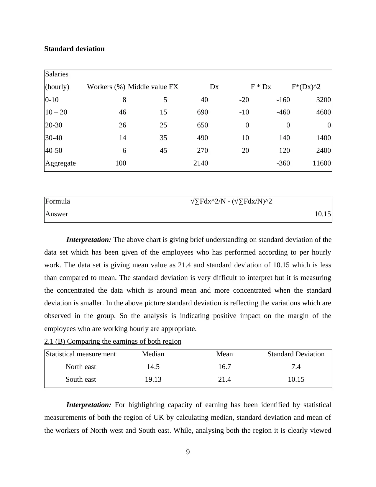
Standard deviation
Salaries
(hourly) Workers (%) Middle value FX Dx F * Dx F*(Dx)^2
0-10 8 5 40 -20 -160 3200
10 – 20 46 15 690 -10 -460 4600
20-30 26 25 650 0 0 0
30-40 14 35 490 10 140 1400
40-50 6 45 270 20 120 2400
Aggregate 100 2140 -360 11600
Formula √∑Fdx^2/N - (√∑Fdx/N)^2
Answer 10.15
Interpretation: The above chart is giving brief understanding on standard deviation of the
data set which has been given of the employees who has performed according to per hourly
work. The data set is giving mean value as 21.4 and standard deviation of 10.15 which is less
than compared to mean. The standard deviation is very difficult to interpret but it is measuring
the concentrated the data which is around mean and more concentrated when the standard
deviation is smaller. In the above picture standard deviation is reflecting the variations which are
observed in the group. So the analysis is indicating positive impact on the margin of the
employees who are working hourly are appropriate.
2.1 (B) Comparing the earnings of both region
Statistical measurement Median Mean Standard Deviation
North east 14.5 16.7 7.4
South east 19.13 21.4 10.15
Interpretation: For highlighting capacity of earning has been identified by statistical
measurements of both the region of UK by calculating median, standard deviation and mean of
the workers of North west and South east. While, analysing both the region it is clearly viewed
9

that there are more efficient employees in South east as compared to North west. The North west
is giving mean value as 16.70 and South east as 21.40, so according to mean value South east is
more indulgent with the context of generating more revenue and better earnings by the workers.
Standard deviation of both regions consists of huge differences as North West is 7.4 and south
east is 10.15. The median analysis of north west is 14.50 and South East is 19.13. The outcomes
are replicating various changes but with the context of median analysis, efficient employees are
in north west and analysing overall, South east region has appropriate growth and will be able to
generate more profit.
Activity 3
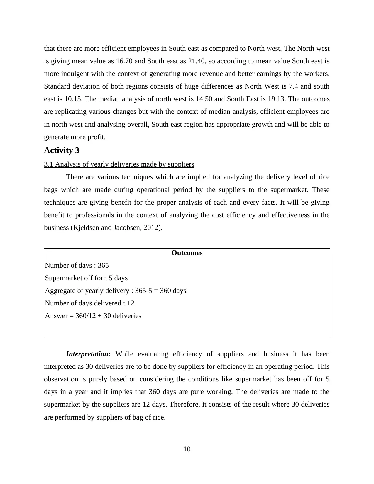
3.1 Analysis of yearly deliveries made by suppliers
There are various techniques which are implied for analyzing the delivery level of rice
bags which are made during operational period by the suppliers to the supermarket. These
techniques are giving benefit for the proper analysis of each and every facts. It will be giving
benefit to professionals in the context of analyzing the cost efficiency and effectiveness in the
business (Kjeldsen and Jacobsen, 2012).
Outcomes
Number of days : 365
Supermarket off for : 5 days
Aggregate of yearly delivery : 365-5 = 360 days
Number of days delivered : 12
Answer = 360/12 + 30 deliveries
Interpretation: While evaluating efficiency of suppliers and business it has been
interpreted as 30 deliveries are to be done by suppliers for efficiency in an operating period. This
observation is purely based on considering the conditions like supermarket has been off for 5
days in a year and it implies that 360 days are pure working. The deliveries are made to the
supermarket by the suppliers are 12 days. Therefore, it consists of the result where 30 deliveries
are performed by suppliers of bag of rice.
10