Statistics: Unit 4 Dropbox Assignment Answers Analysis and Results

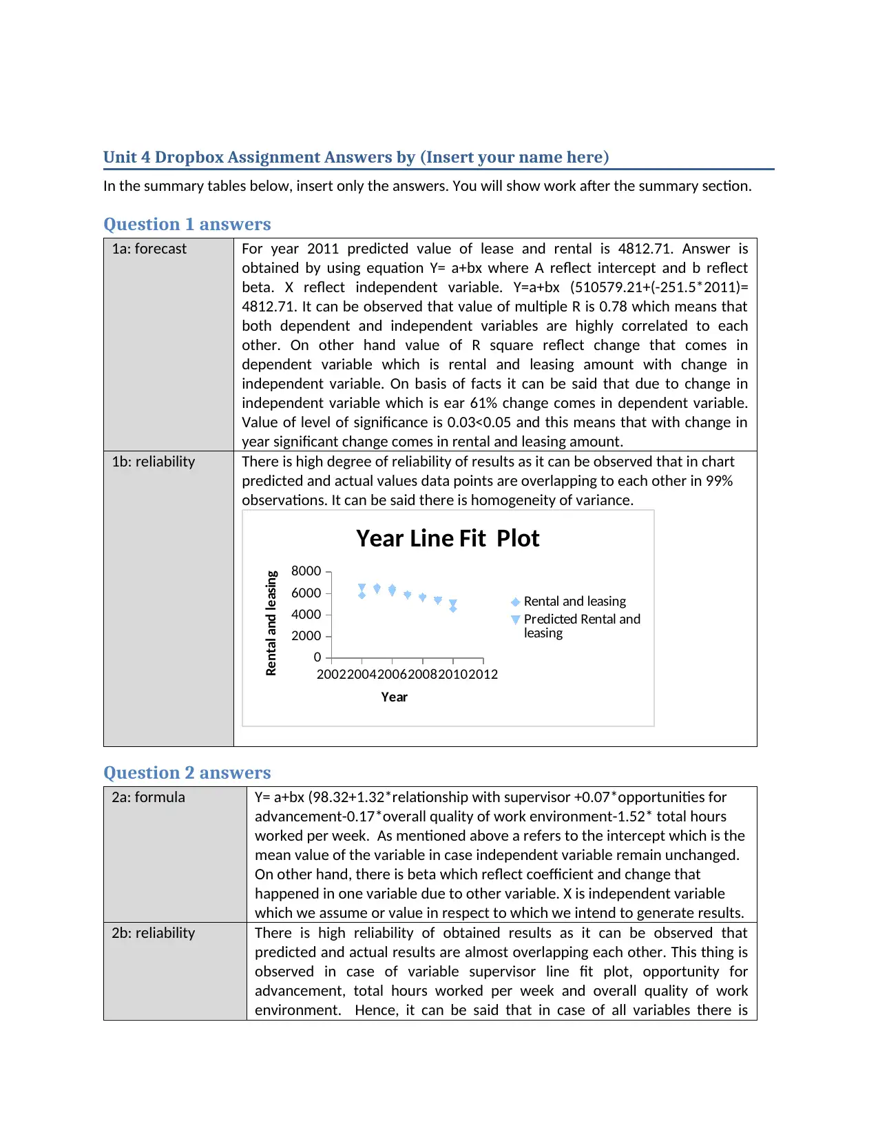
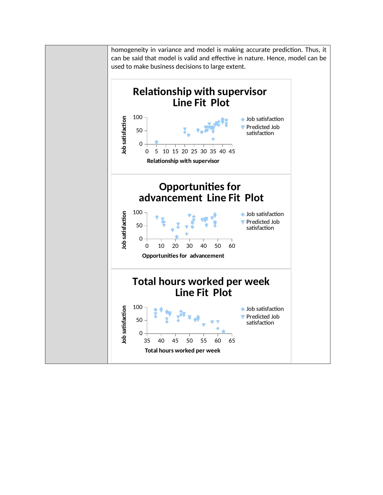
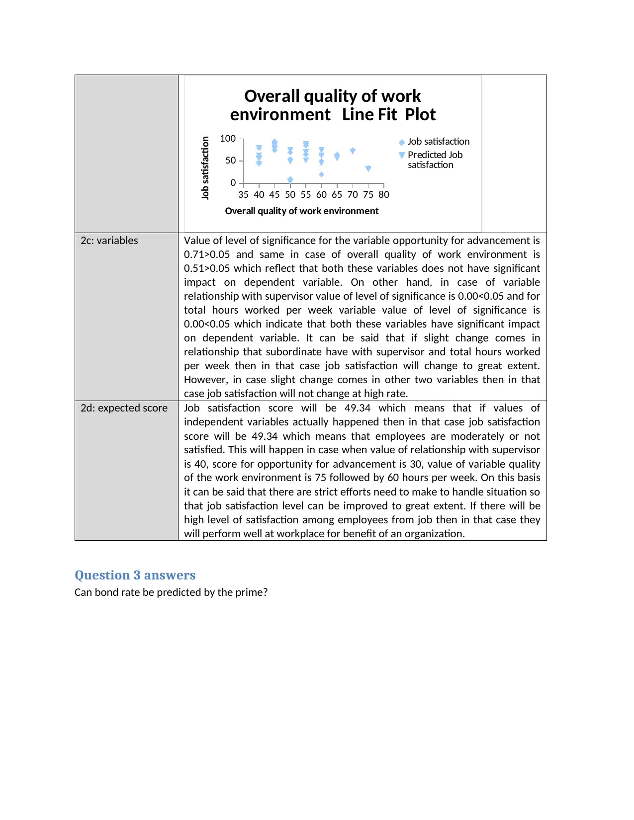
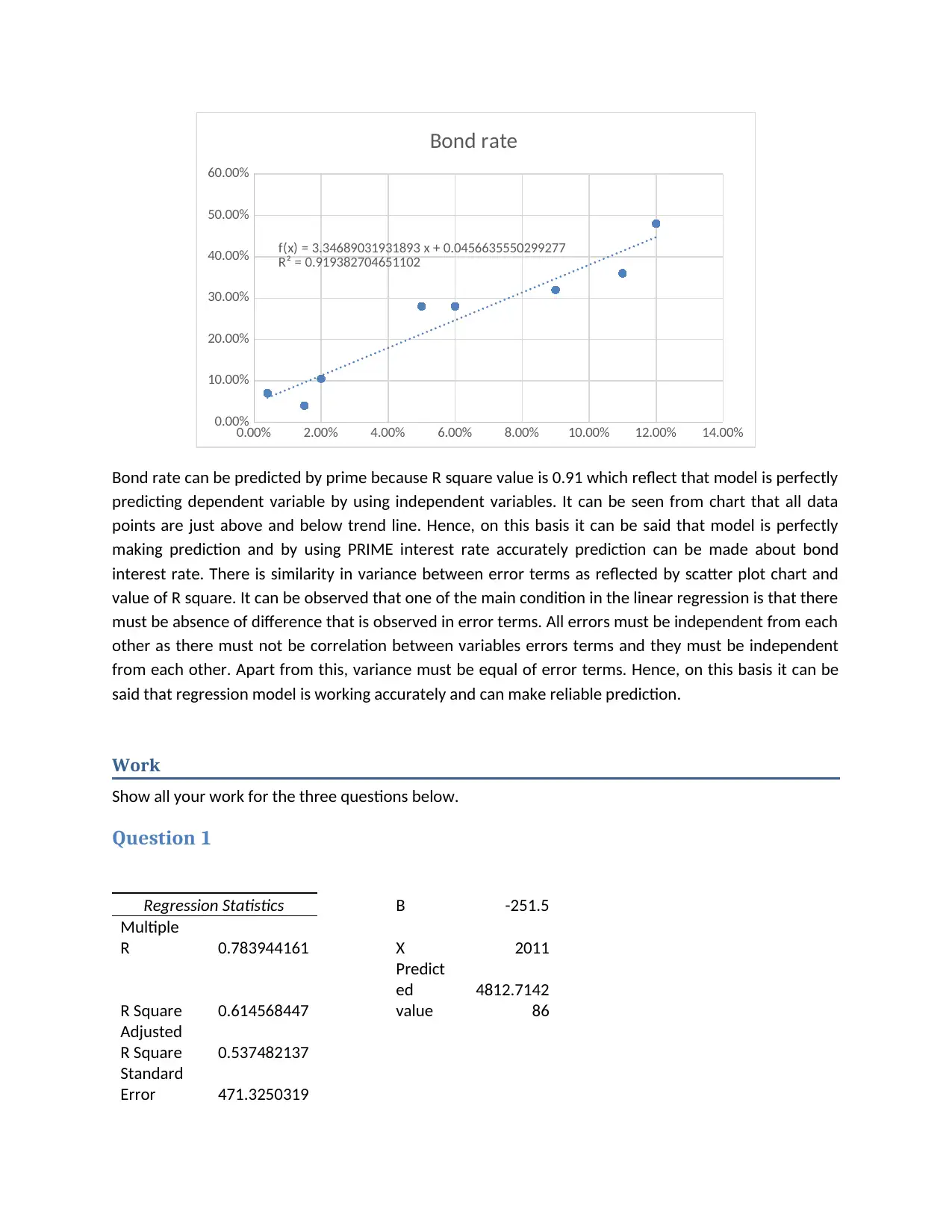
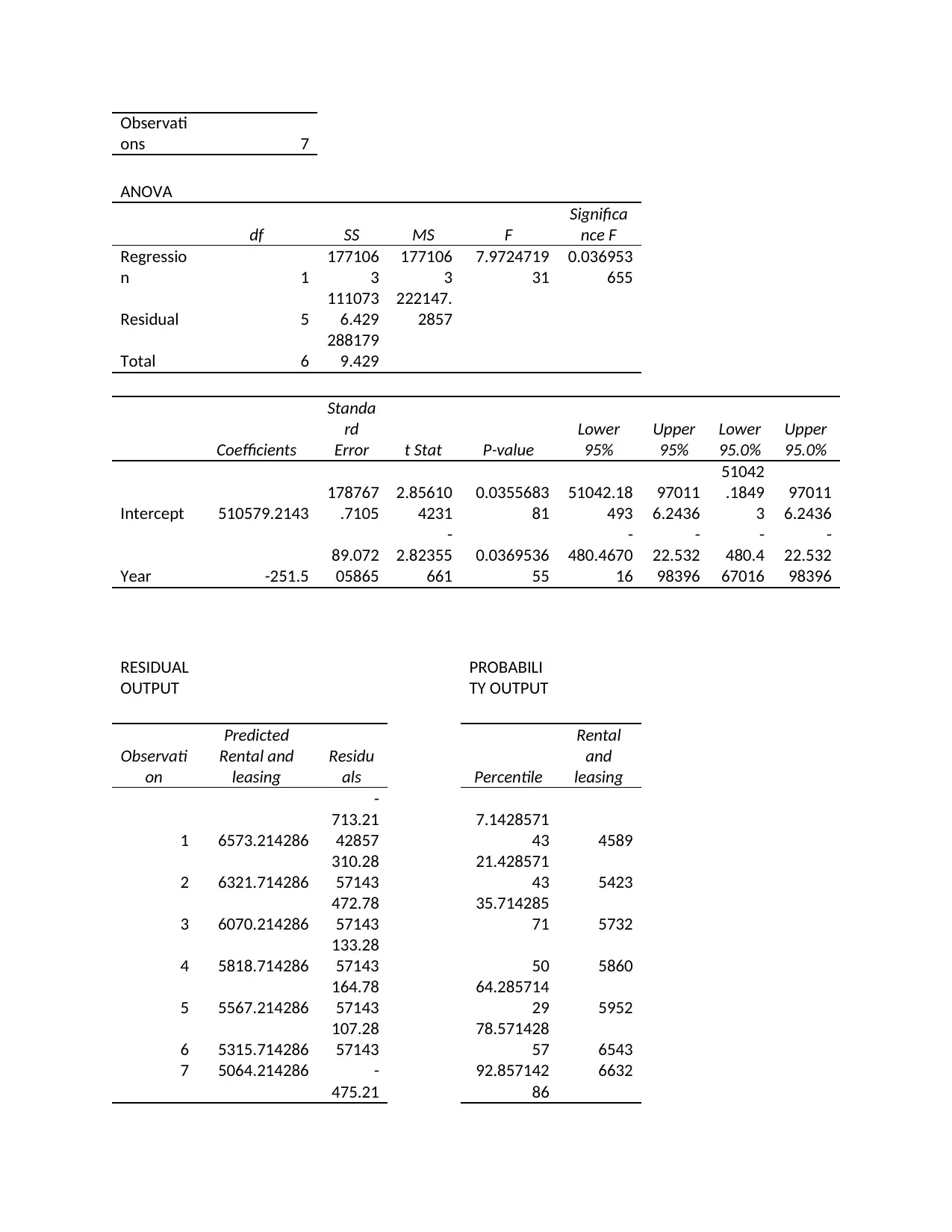
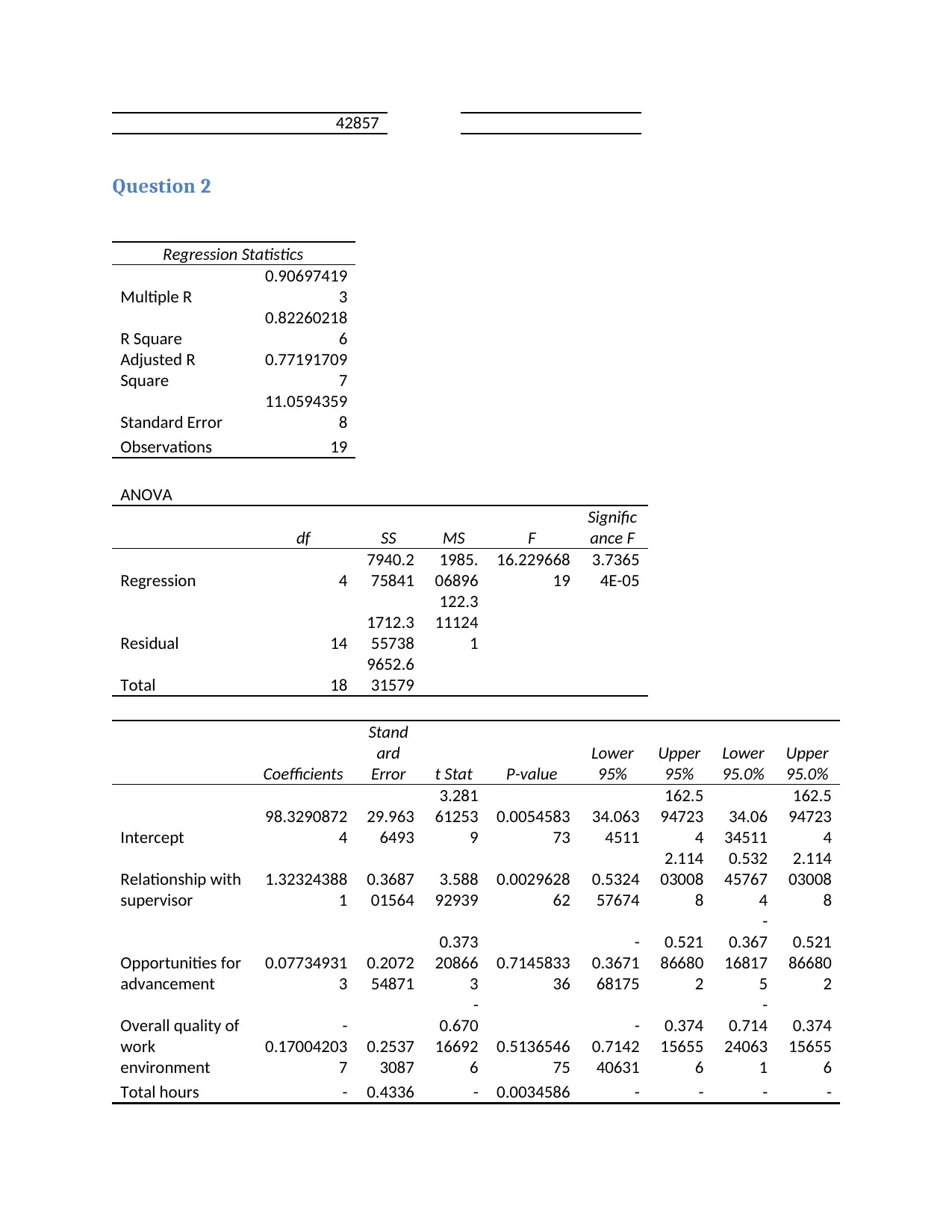
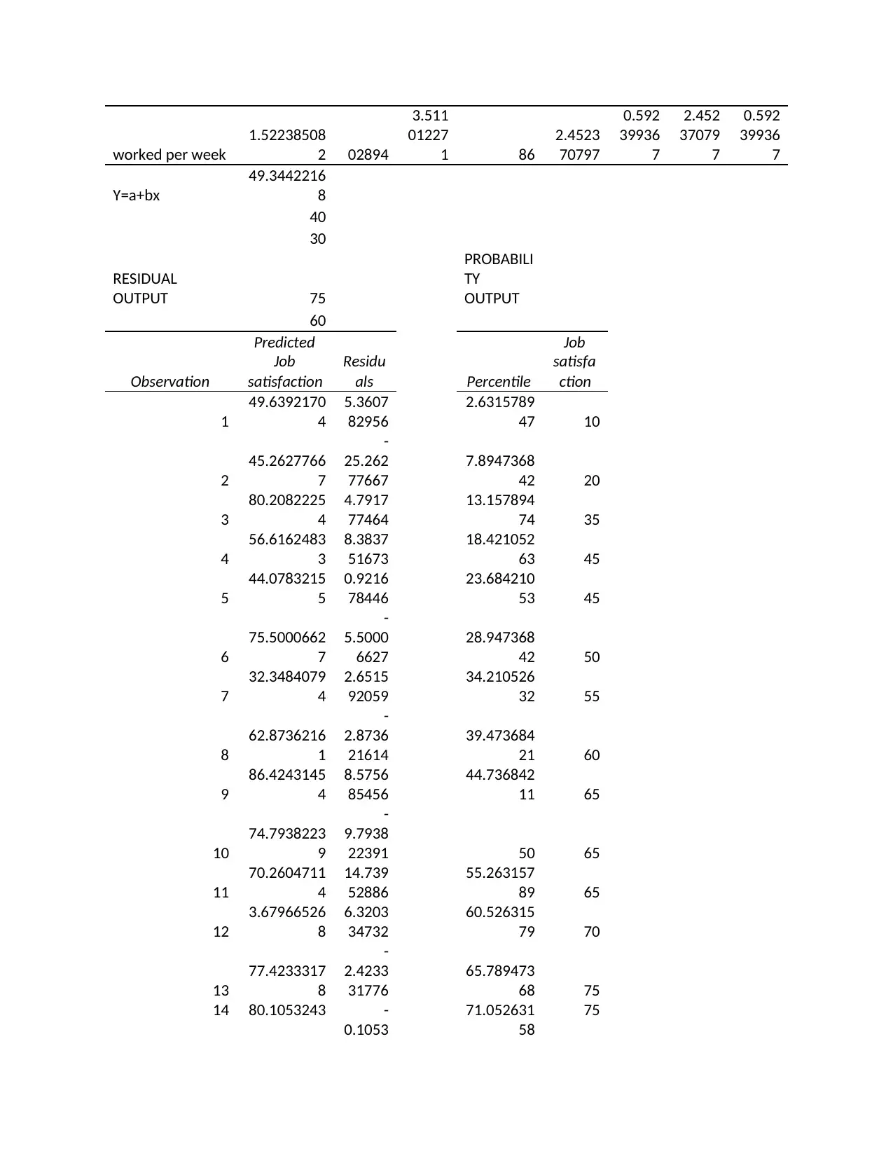
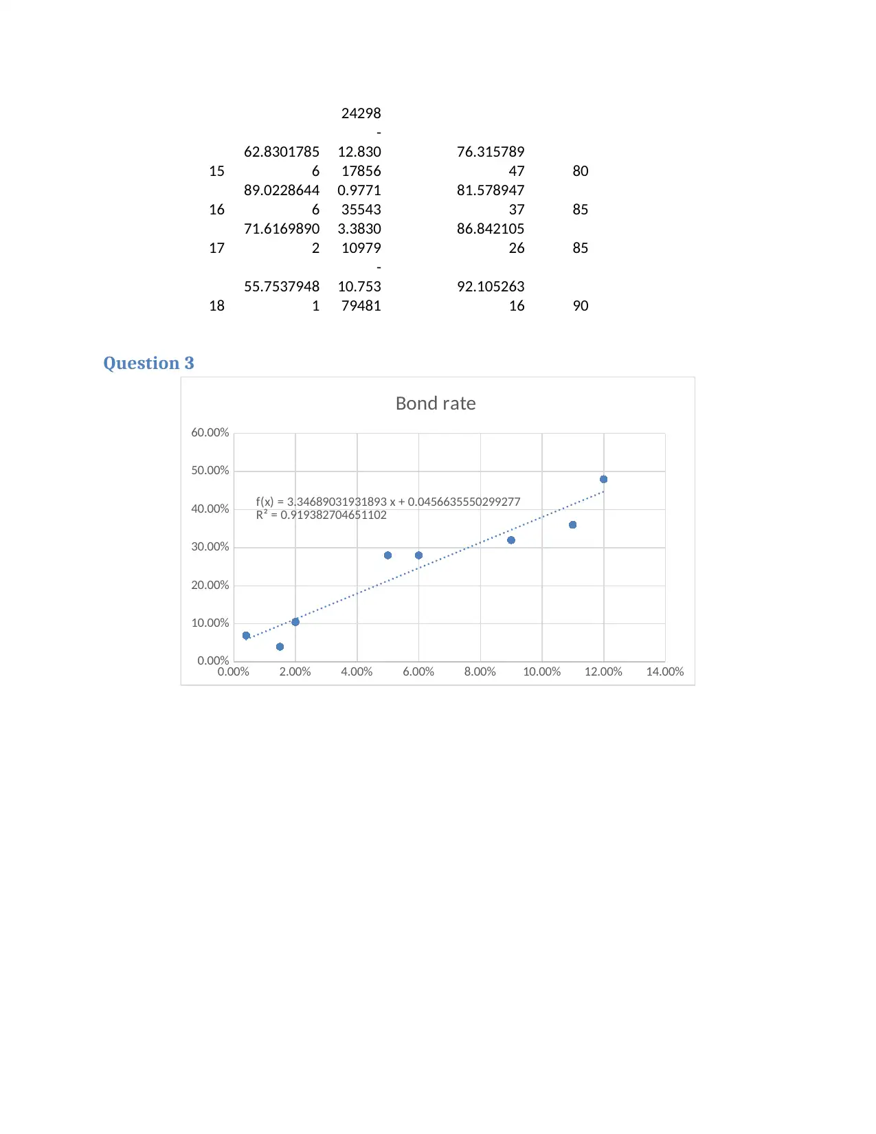
This document presents solutions to a statistics assignment, focusing on regression analysis and its applications. The assignment covers three questions, each involving statistical modeling and interpretation. Question 1 addresses forecasting using linear regression, predicting lease and rental values based on historical data. Question 2 delves into multiple regression to analyze factors influencing job satisfaction, evaluating the significance of variables like supervisor relationships, opportunities for advancement, and work environment. Question 3 explores the prediction of bond rates using prime interest rates, assessing the model's reliability and validity through R-squared values and scatter plot analysis. The solutions include formulas, statistical outputs, and detailed interpretations of the results, including ANOVA tables and regression statistics, providing a comprehensive understanding of the statistical concepts applied. The document also discusses the reliability of results, the impact of different variables, and expected scores. The work includes detailed calculations and analysis for all three questions.

Unit 4 Dropbox Assignment Answers by (Insert your name here)
In the summary tables below, insert only the answers. You will show work after the summary section.
Question 1 answers
1a: forecast For year 2011 predicted value of lease and rental is 4812.71. Answer is
obtained by using equation Y= a+bx where A reflect intercept and b reflect
beta. X reflect independent variable. Y=a+bx (510579.21+(-251.5*2011)=
4812.71. It can be observed that value of multiple R is 0.78 which means that
both dependent and independent variables are highly correlated to each
other. On other hand value of R square reflect change that comes in
dependent variable which is rental and leasing amount with change in
independent variable. On basis of facts it can be said that due to change in
independent variable which is ear 61% change comes in dependent variable.
Value of level of significance is 0.03<0.05 and this means that with change in
year significant change comes in rental and leasing amount.
1b: reliability There is high degree of reliability of results as it can be observed that in chart
predicted and actual values data points are overlapping to each other in 99%
observations. It can be said there is homogeneity of variance.
200220042006200820102012
0
2000
4000
6000
8000
Year Line Fit Plot
Rental and leasing
Predicted Rental and
leasing
Year
Rental and leasing
Question 2 answers
2a: formula Y= a+bx (98.32+1.32*relationship with supervisor +0.07*opportunities for
advancement-0.17*overall quality of work environment-1.52* total hours
worked per week. As mentioned above a refers to the intercept which is the
mean value of the variable in case independent variable remain unchanged.
On other hand, there is beta which reflect coefficient and change that
happened in one variable due to other variable. X is independent variable
which we assume or value in respect to which we intend to generate results.
2b: reliability There is high reliability of obtained results as it can be observed that
predicted and actual results are almost overlapping each other. This thing is
observed in case of variable supervisor line fit plot, opportunity for
advancement, total hours worked per week and overall quality of work
environment. Hence, it can be said that in case of all variables there is

homogeneity in variance and model is making accurate prediction. Thus, it
can be said that model is valid and effective in nature. Hence, model can be
used to make business decisions to large extent.
0 5 10 15 20 25 30 35 40 45
0
50
100
Relationship with supervisor
Line Fit Plot
Job satisfaction
Predicted Job
satisfaction
Relationship with supervisor
Job satisfaction
0 10 20 30 40 50 60
0
50
100
Opportunities for
advancement Line Fit Plot
Job satisfaction
Predicted Job
satisfaction
Opportunities for advancement
Job satisfaction
35 40 45 50 55 60 65
0
50
100
Total hours worked per week
Line Fit Plot
Job satisfaction
Predicted Job
satisfaction
Total hours worked per week
Job satisfaction

35 40 45 50 55 60 65 70 75 80
0
50
100
Overall quality of work
environment Line Fit Plot
Job satisfaction
Predicted Job
satisfaction
Overall quality of work environment
Job satisfaction
2c: variables Value of level of significance for the variable opportunity for advancement is
0.71>0.05 and same in case of overall quality of work environment is
0.51>0.05 which reflect that both these variables does not have significant
impact on dependent variable. On other hand, in case of variable
relationship with supervisor value of level of significance is 0.00<0.05 and for
total hours worked per week variable value of level of significance is
0.00<0.05 which indicate that both these variables have significant impact
on dependent variable. It can be said that if slight change comes in
relationship that subordinate have with supervisor and total hours worked
per week then in that case job satisfaction will change to great extent.
However, in case slight change comes in other two variables then in that
case job satisfaction will not change at high rate.
2d: expected score Job satisfaction score will be 49.34 which means that if values of
independent variables actually happened then in that case job satisfaction
score will be 49.34 which means that employees are moderately or not
satisfied. This will happen in case when value of relationship with supervisor
is 40, score for opportunity for advancement is 30, value of variable quality
of the work environment is 75 followed by 60 hours per week. On this basis
it can be said that there are strict efforts need to make to handle situation so
that job satisfaction level can be improved to great extent. If there will be
high level of satisfaction among employees from job then in that case they
will perform well at workplace for benefit of an organization.
Question 3 answers
Can bond rate be predicted by the prime?

0.00% 2.00% 4.00% 6.00% 8.00% 10.00% 12.00% 14.00%
0.00%
10.00%
20.00%
30.00%
40.00%
50.00%
60.00%
f(x) = 3.34689031931893 x + 0.0456635550299277
R² = 0.919382704651102
Bond rate
Bond rate can be predicted by prime because R square value is 0.91 which reflect that model is perfectly
predicting dependent variable by using independent variables. It can be seen from chart that all data
points are just above and below trend line. Hence, on this basis it can be said that model is perfectly
making prediction and by using PRIME interest rate accurately prediction can be made about bond
interest rate. There is similarity in variance between error terms as reflected by scatter plot chart and
value of R square. It can be observed that one of the main condition in the linear regression is that there
must be absence of difference that is observed in error terms. All errors must be independent from each
other as there must not be correlation between variables errors terms and they must be independent
from each other. Apart from this, variance must be equal of error terms. Hence, on this basis it can be
said that regression model is working accurately and can make reliable prediction.
Work
Show all your work for the three questions below.
Question 1
Regression Statistics B -251.5
Multiple
R 0.783944161 X 2011
R Square 0.614568447
Predict
ed
value
4812.7142
86
Adjusted
R Square 0.537482137
Standard
Error 471.3250319

Observati
ons 7
ANOVA
df SS MS F
Significa
nce F
Regressio
n 1
177106
3
177106
3
7.9724719
31
0.036953
655
Residual 5
111073
6.429
222147.
2857
Total 6
288179
9.429
Coefficients
Standa
rd
Error t Stat P-value
Lower
95%
Upper
95%
Lower
95.0%
Upper
95.0%
Intercept 510579.2143
178767
.7105
2.85610
4231
0.0355683
81
51042.18
493
97011
6.2436
51042
.1849
3
97011
6.2436
Year -251.5
89.072
05865
-
2.82355
661
0.0369536
55
-
480.4670
16
-
22.532
98396
-
480.4
67016
-
22.532
98396
RESIDUAL
OUTPUT
PROBABILI
TY OUTPUT
Observati
on
Predicted
Rental and
leasing
Residu
als Percentile
Rental
and
leasing
1 6573.214286
-
713.21
42857
7.1428571
43 4589
2 6321.714286
310.28
57143
21.428571
43 5423
3 6070.214286
472.78
57143
35.714285
71 5732
4 5818.714286
133.28
57143 50 5860
5 5567.214286
164.78
57143
64.285714
29 5952
6 5315.714286
107.28
57143
78.571428
57 6543
7 5064.214286 -
475.21
92.857142
86
6632

42857
Question 2
Regression Statistics
Multiple R
0.90697419
3
R Square
0.82260218
6
Adjusted R
Square
0.77191709
7
Standard Error
11.0594359
8
Observations 19
ANOVA
df SS MS F
Signific
ance F
Regression 4
7940.2
75841
1985.
06896
16.229668
19
3.7365
4E-05
Residual 14
1712.3
55738
122.3
11124
1
Total 18
9652.6
31579
Coefficients
Stand
ard
Error t Stat P-value
Lower
95%
Upper
95%
Lower
95.0%
Upper
95.0%
Intercept
98.3290872
4
29.963
6493
3.281
61253
9
0.0054583
73
34.063
4511
162.5
94723
4
34.06
34511
162.5
94723
4
Relationship with
supervisor
1.32324388
1
0.3687
01564
3.588
92939
0.0029628
62
0.5324
57674
2.114
03008
8
0.532
45767
4
2.114
03008
8
Opportunities for
advancement
0.07734931
3
0.2072
54871
0.373
20866
3
0.7145833
36
-
0.3671
68175
0.521
86680
2
-
0.367
16817
5
0.521
86680
2
Overall quality of
work
environment
-
0.17004203
7
0.2537
3087
-
0.670
16692
6
0.5136546
75
-
0.7142
40631
0.374
15655
6
-
0.714
24063
1
0.374
15655
6
Total hours - 0.4336 - 0.0034586 - - - -

worked per week
1.52238508
2 02894
3.511
01227
1 86
2.4523
70797
0.592
39936
7
2.452
37079
7
0.592
39936
7
Y=a+bx
49.3442216
8
40
30
RESIDUAL
OUTPUT 75
PROBABILI
TY
OUTPUT
60
Observation
Predicted
Job
satisfaction
Residu
als Percentile
Job
satisfa
ction
1
49.6392170
4
5.3607
82956
2.6315789
47 10
2
45.2627766
7
-
25.262
77667
7.8947368
42 20
3
80.2082225
4
4.7917
77464
13.157894
74 35
4
56.6162483
3
8.3837
51673
18.421052
63 45
5
44.0783215
5
0.9216
78446
23.684210
53 45
6
75.5000662
7
-
5.5000
6627
28.947368
42 50
7
32.3484079
4
2.6515
92059
34.210526
32 55
8
62.8736216
1
-
2.8736
21614
39.473684
21 60
9
86.4243145
4
8.5756
85456
44.736842
11 65
10
74.7938223
9
-
9.7938
22391 50 65
11
70.2604711
4
14.739
52886
55.263157
89 65
12
3.67966526
8
6.3203
34732
60.526315
79 70
13
77.4233317
8
-
2.4233
31776
65.789473
68 75
14 80.1053243 -
0.1053
71.052631
58
75

24298
15
62.8301785
6
-
12.830
17856
76.315789
47 80
16
89.0228644
6
0.9771
35543
81.578947
37 85
17
71.6169890
2
3.3830
10979
86.842105
26 85
18
55.7537948
1
-
10.753
79481
92.105263
16 90
Question 3
0.00% 2.00% 4.00% 6.00% 8.00% 10.00% 12.00% 14.00%
0.00%
10.00%
20.00%
30.00%
40.00%
50.00%
60.00%
f(x) = 3.34689031931893 x + 0.0456635550299277
R² = 0.919382704651102
Bond rate