Detailed Solution to Statistics 630 Assignment 3: Probability Theory

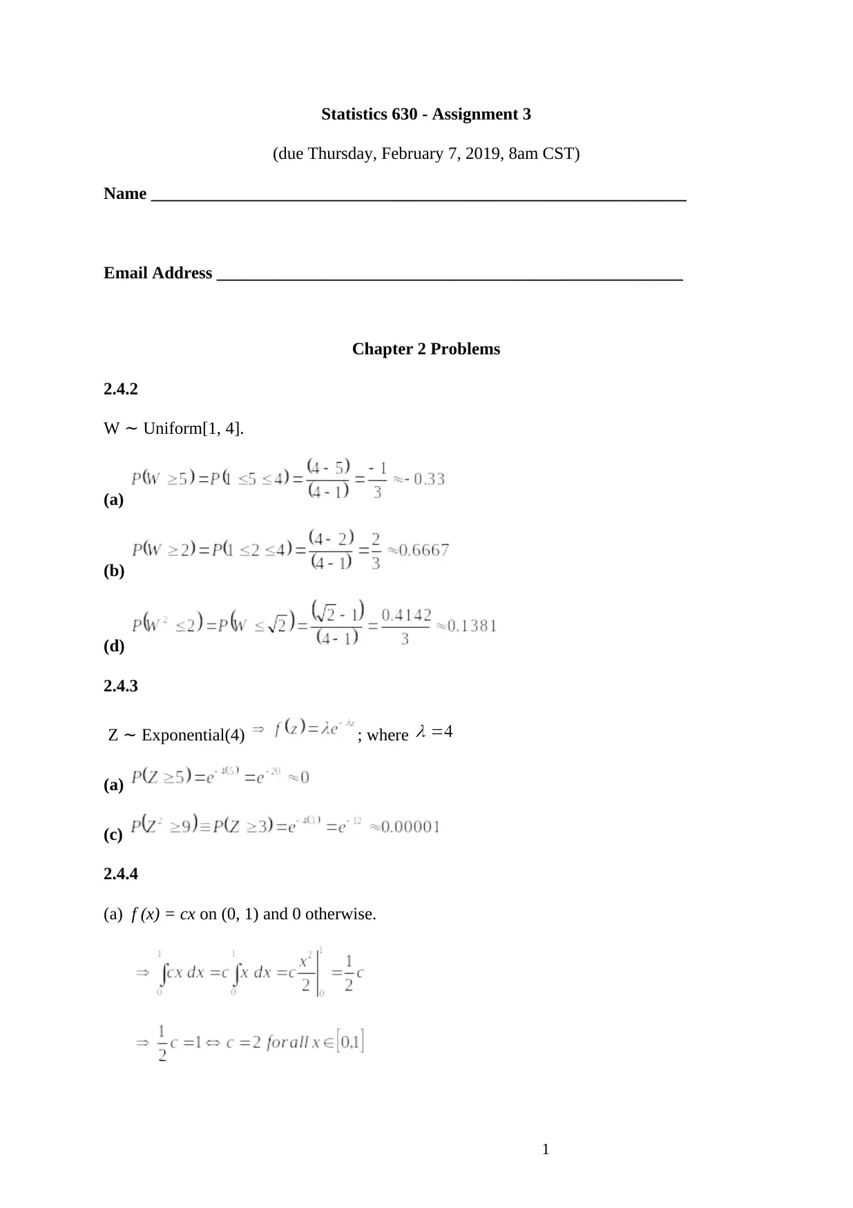
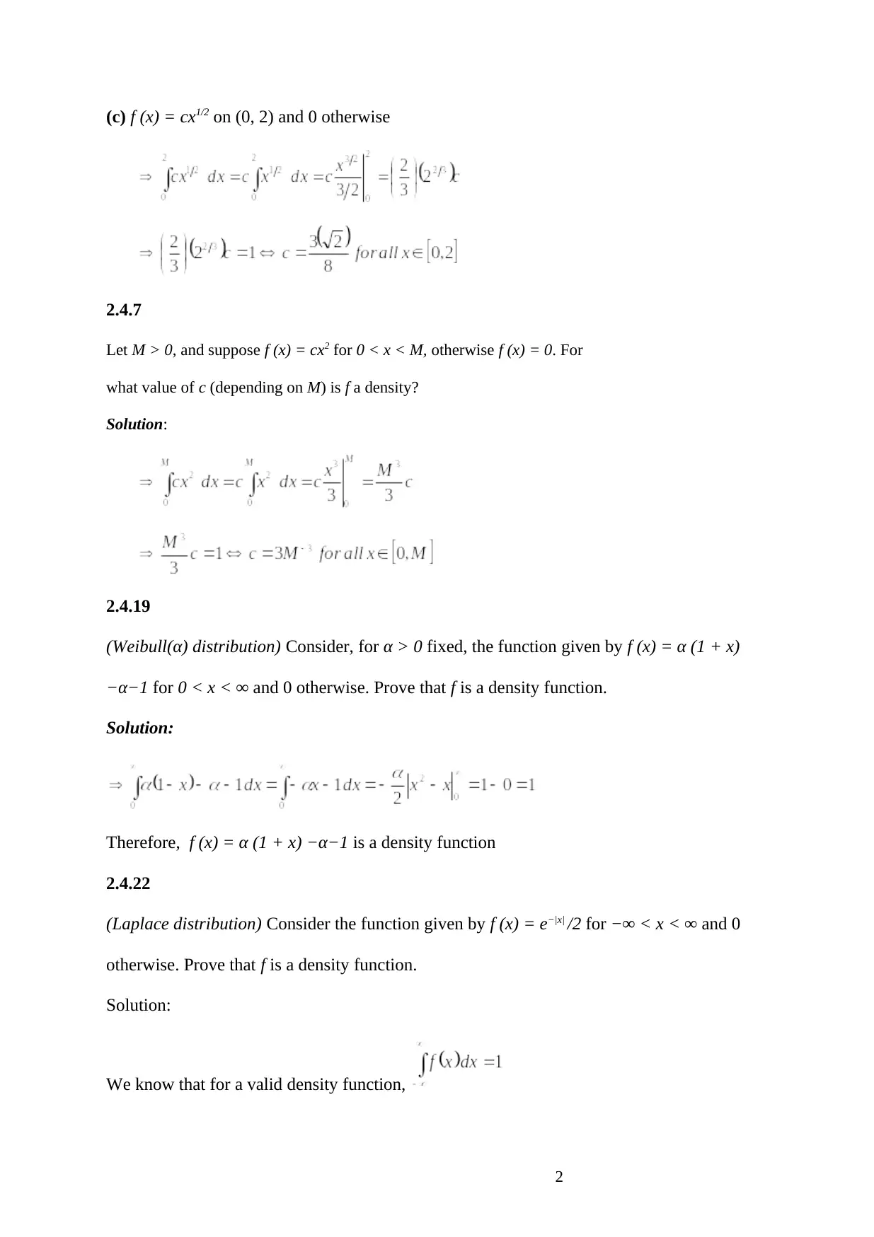
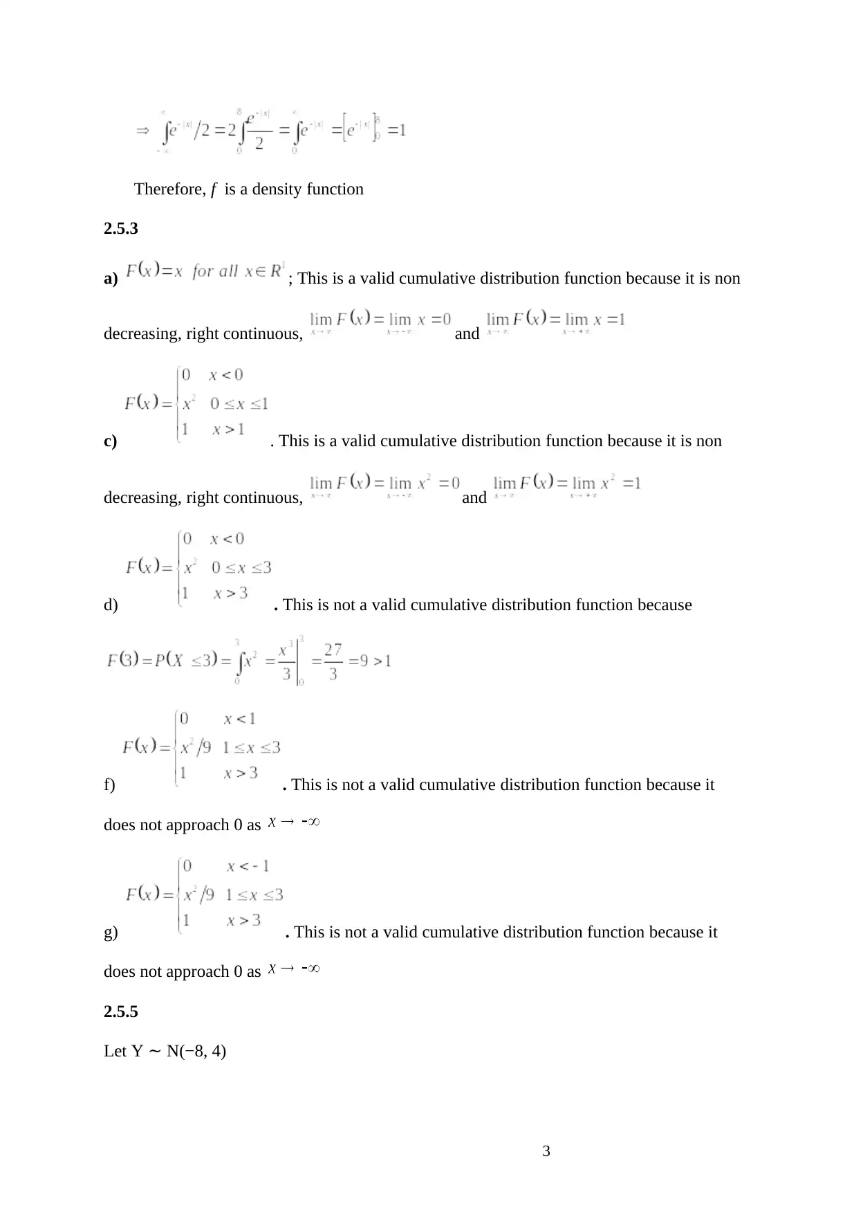
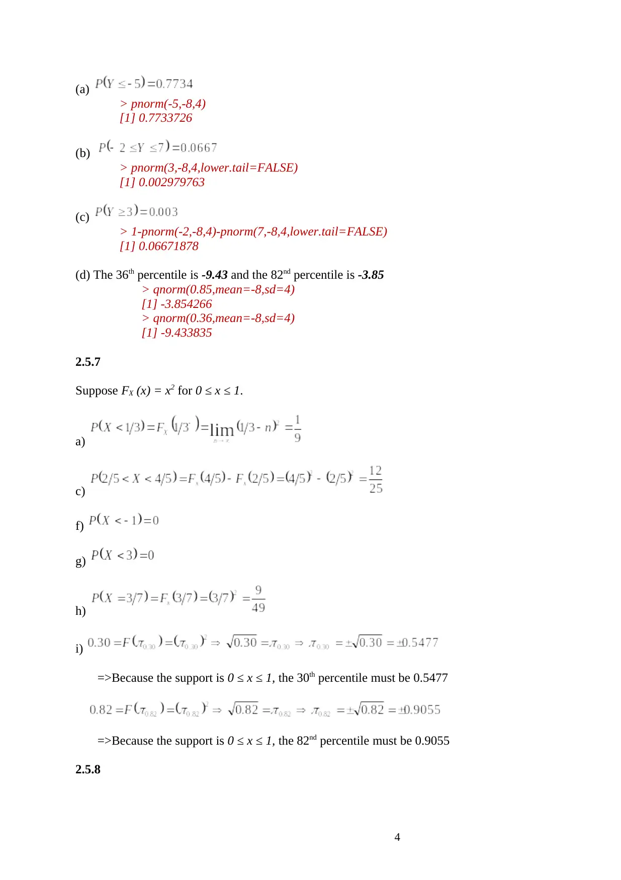
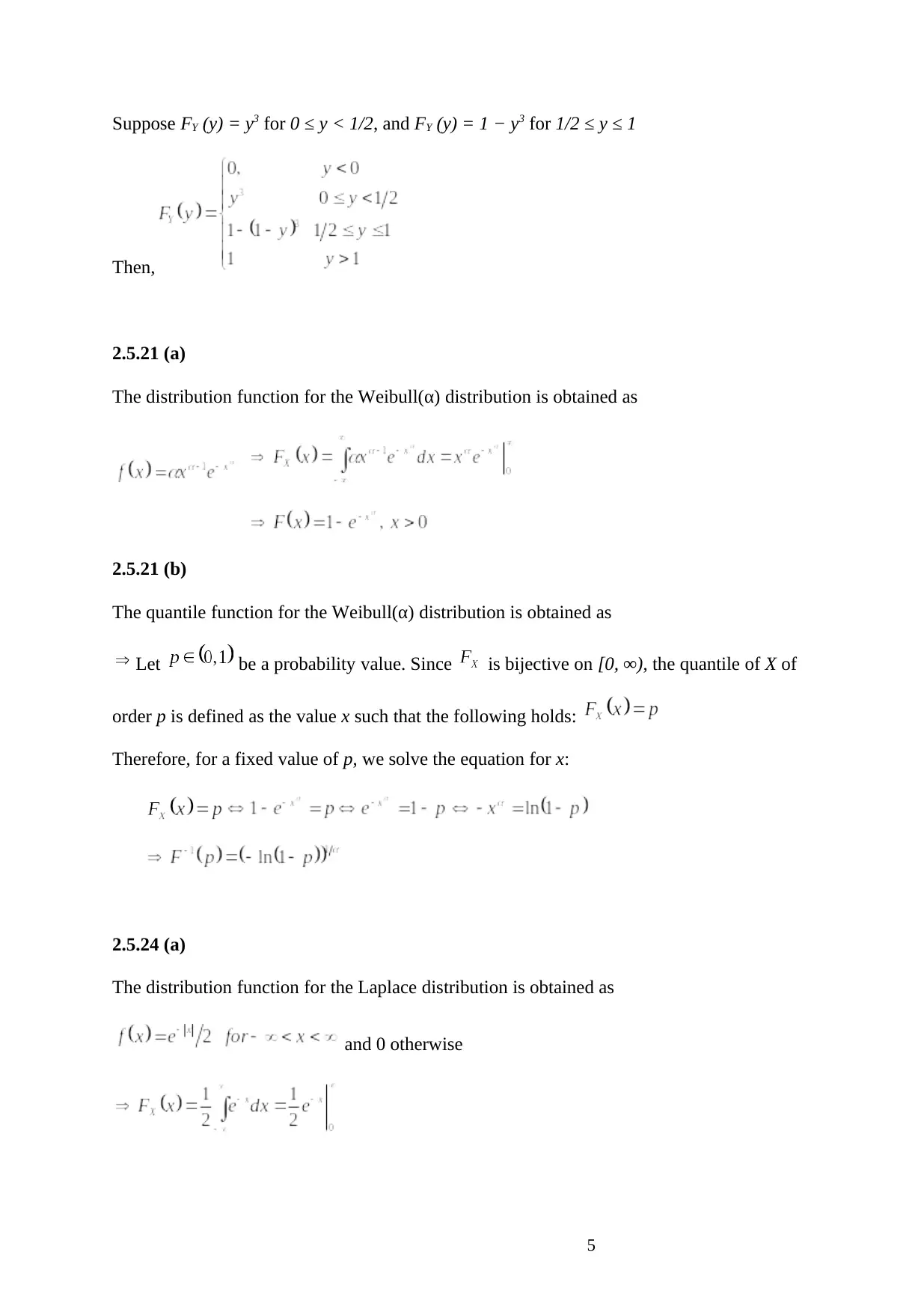
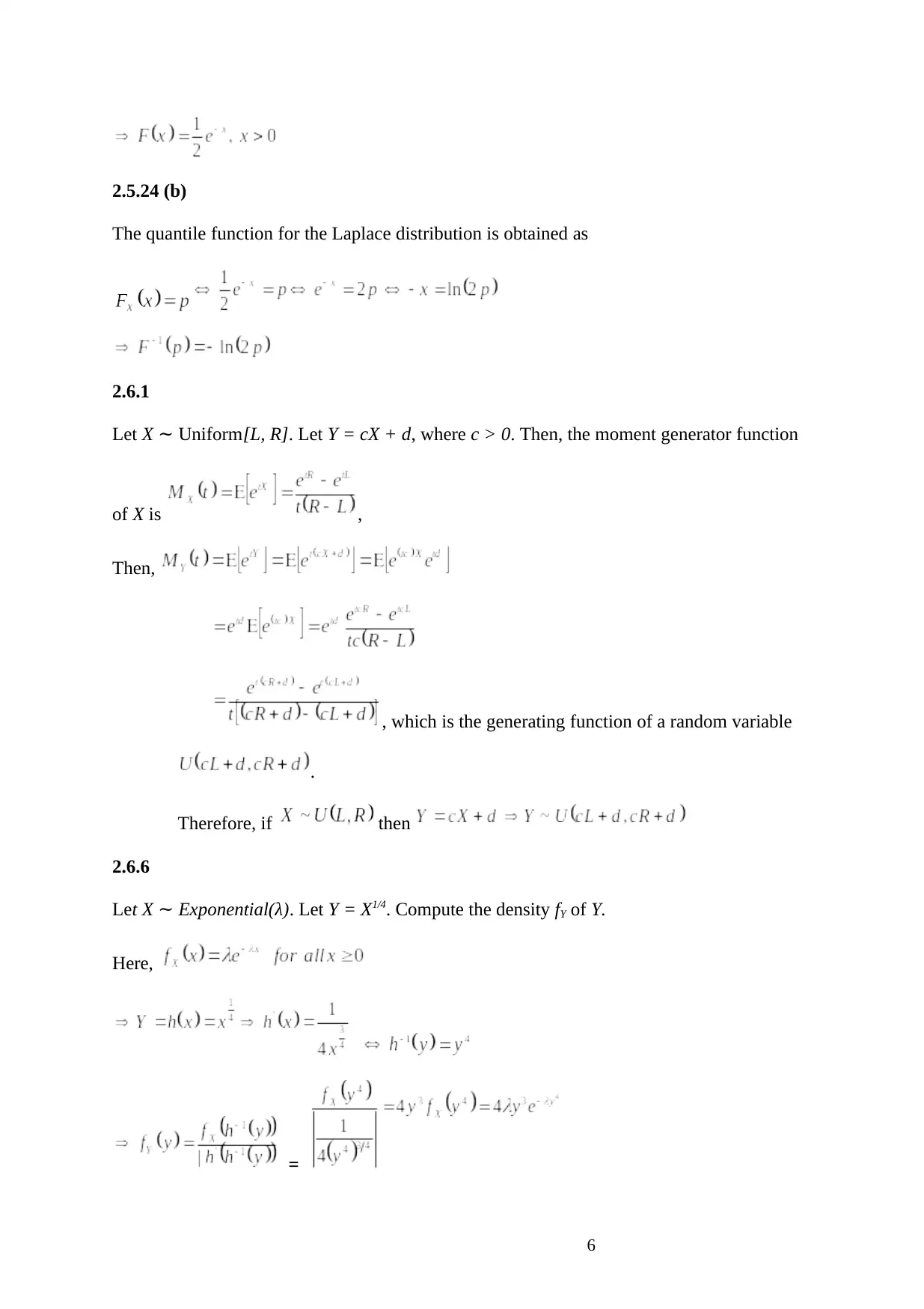
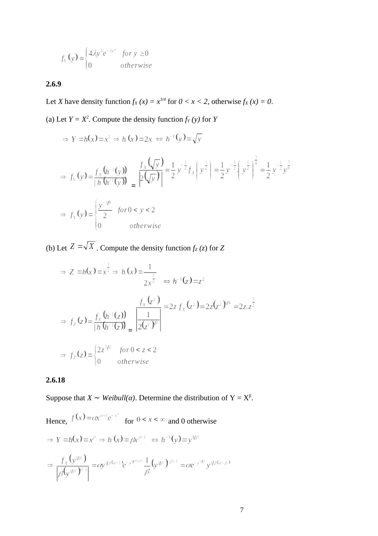
This document presents detailed solutions to the problems in Statistics 630 Assignment 3, focusing on various aspects of probability theory. The solutions cover problems related to uniform, exponential, Weibull, and Laplace distributions, including proving density functions and computing cumulative distribution functions. Additionally, the assignment explores quantile functions, moment generating functions, and transformations of random variables. Specific problems include finding the density function of Y = X^(1/4) when X follows an exponential distribution, determining the distribution of Y = X^β when X follows a Weibull distribution, and validating cumulative distribution functions. The solutions are comprehensive and provide step-by-step explanations, making it a valuable resource for students studying probability and statistics. Desklib provides access to this and other solved assignments to aid student learning.

1
Statistics 630 - Assignment 3
(due Thursday, February 7, 2019, 8am CST)
Name ______________________________________________________________
Email Address ______________________________________________________
Chapter 2 Problems
2.4.2
W Uniform[1, 4].∼
(a)
(b)
(d)
2.4.3
Z Exponential(4)∼ ; where
(a)
(c)
2.4.4
(a) f (x) = cx on (0, 1) and 0 otherwise.

2
(c) f (x) = cx1/2 on (0, 2) and 0 otherwise
2.4.7
Let M > 0, and suppose f (x) = cx2 for 0 < x < M, otherwise f (x) = 0. For
what value of c (depending on M) is f a density?
Solution:
2.4.19
(Weibull(α) distribution) Consider, for α > 0 fixed, the function given by f (x) = α (1 + x)
−α−1 for 0 < x < ∞ and 0 otherwise. Prove that f is a density function.
Solution:
Therefore, f (x) = α (1 + x) −α−1 is a density function
2.4.22
(Laplace distribution) Consider the function given by f (x) = e−|x| /2 for −∞ < x < ∞ and 0
otherwise. Prove that f is a density function.
Solution:
We know that for a valid density function,

3
Therefore, f is a density function
2.5.3
a) ; This is a valid cumulative distribution function because it is non
decreasing, right continuous, and
c) . This is a valid cumulative distribution function because it is non
decreasing, right continuous, and
d) . This is not a valid cumulative distribution function because
f) . This is not a valid cumulative distribution function because it
does not approach 0 as
g) . This is not a valid cumulative distribution function because it
does not approach 0 as
2.5.5
Let Y N(−8, 4)∼

4
(a)
> pnorm(-5,-8,4)
[1] 0.7733726
(b)
> pnorm(3,-8,4,lower.tail=FALSE)
[1] 0.002979763
(c)
> 1-pnorm(-2,-8,4)-pnorm(7,-8,4,lower.tail=FALSE)
[1] 0.06671878
(d) The 36th percentile is -9.43 and the 82nd percentile is -3.85
> qnorm(0.85,mean=-8,sd=4)
[1] -3.854266
> qnorm(0.36,mean=-8,sd=4)
[1] -9.433835
2.5.7
Suppose FX (x) = x2 for 0 ≤ x ≤ 1.
a)
c)
f)
g)
h)
i)
=>Because the support is 0 ≤ x ≤ 1, the 30th percentile must be 0.5477
=>Because the support is 0 ≤ x ≤ 1, the 82nd percentile must be 0.9055
2.5.8

5
Suppose FY (y) = y3 for 0 ≤ y < 1/2, and FY (y) = 1 − y3 for 1/2 ≤ y ≤ 1
Then,
2.5.21 (a)
The distribution function for the Weibull(α) distribution is obtained as
2.5.21 (b)
The quantile function for the Weibull(α) distribution is obtained as
Let be a probability value. Since is bijective on [0, ∞), the quantile of X of
order p is defined as the value x such that the following holds:
Therefore, for a fixed value of p, we solve the equation for x:
2.5.24 (a)
The distribution function for the Laplace distribution is obtained as
and 0 otherwise

6
2.5.24 (b)
The quantile function for the Laplace distribution is obtained as
2.6.1
Let X ∼ Uniform[L, R]. Let Y = cX + d, where c > 0. Then, the moment generator function
of X is ,
Then,
, which is the generating function of a random variable
.
Therefore, if then
2.6.6
Let X Exponential(λ)∼ . Let Y = X1/4. Compute the density fY of Y.
Here,
=

7
2.6.9
Let X have density function fX (x) = x3/4 for 0 < x < 2, otherwise fX (x) = 0.
(a) Let Y = X2. Compute the density function fY (y) for Y
=
(b) Let . Compute the density function fZ (z) for Z
=
2.6.18
Suppose that X Weibull(α)∼ . Determine the distribution of Y = Xβ.
Hence, for and 0 otherwise

8