Statistical Analysis: Confidence Intervals and Hypothesis Testing

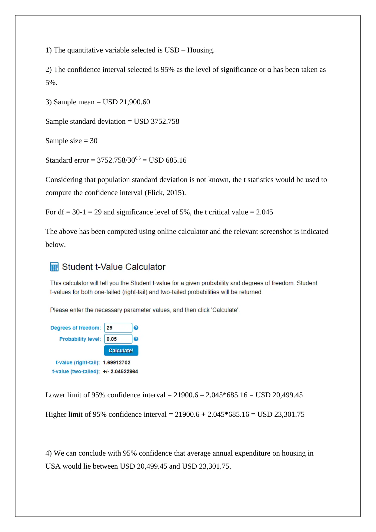
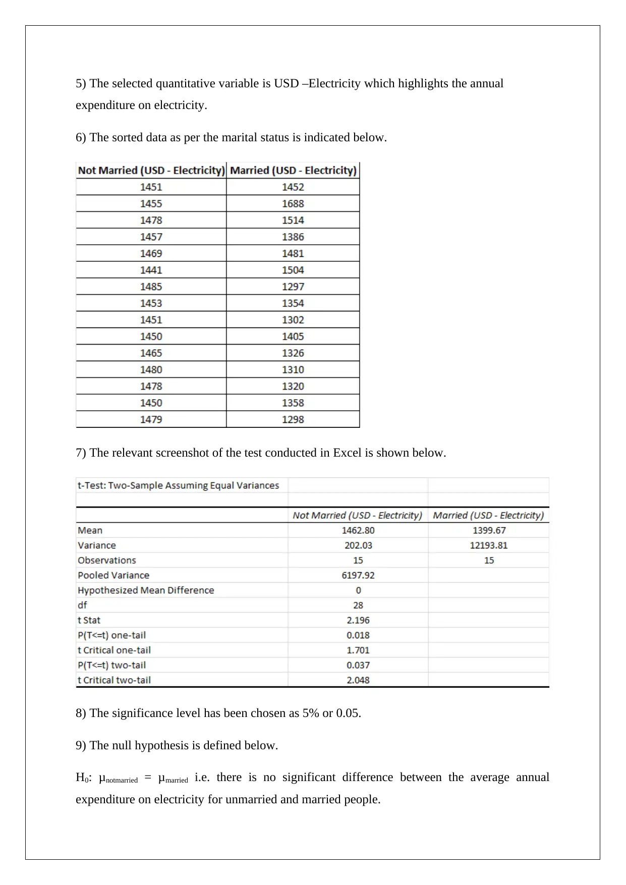
This statistics assignment solution involves calculating a 95% confidence interval for average annual housing expenditure in the USA, determining it to be between USD 20,499.45 and USD 23,301.75 using a t-statistic. It also explores the difference in average annual electricity expenditure between married and unmarried individuals using a two-independent samples hypothesis test. The null hypothesis, stating no significant difference, is rejected based on a p-value of 0.037, leading to the conclusion that there is a statistically significant difference in electricity spending between the two groups. The solution includes relevant calculations, screenshots, and references to support the analysis.

STATISTICS
STUDENT ID:
[Pick the date]

1) The quantitative variable selected is USD – Housing.
2) The confidence interval selected is 95% as the level of significance or α has been taken as
5%.
3) Sample mean = USD 21,900.60
Sample standard deviation = USD 3752.758
Sample size = 30
Standard error = 3752.758/300.5 = USD 685.16
Considering that population standard deviation is not known, the t statistics would be used to
compute the confidence interval (Flick, 2015).
For df = 30-1 = 29 and significance level of 5%, the t critical value = 2.045
The above has been computed using online calculator and the relevant screenshot is indicated
below.
Lower limit of 95% confidence interval = 21900.6 – 2.045*685.16 = USD 20,499.45
Higher limit of 95% confidence interval = 21900.6 + 2.045*685.16 = USD 23,301.75
4) We can conclude with 95% confidence that average annual expenditure on housing in
USA would lie between USD 20,499.45 and USD 23,301.75.

5) The selected quantitative variable is USD –Electricity which highlights the annual
expenditure on electricity.
6) The sorted data as per the marital status is indicated below.
7) The relevant screenshot of the test conducted in Excel is shown below.
8) The significance level has been chosen as 5% or 0.05.
9) The null hypothesis is defined below.
H0: μnotmarried = μmarried i.e. there is no significant difference between the average annual
expenditure on electricity for unmarried and married people.

10) The alternative hypothesis is defined below.
H1: μnotmarried ≠ μmarried i.e. there is significant difference between the average annual
expenditure on electricity for unmarried and married people.
11) The relevant test statistic t is 2.196.
12) Considering that the given hypothesis test is two tailed as is apparent from the alternative
hypothesis, hence the p value is 0.037 (Hair, Wolfinbarger, Money, Samouel & Page,2015).
13) As the computed p value(0.037) tends to be lesser than the corresponding significance
level (0.05), hence it would be appropriate to reject the null hypothesis. Since the null
hypothesis is rejected, hence the alternative hypothesis would be accepted (Hillier, 2016).
14) Thus, the conclusion is that there is difference between the average annual electricity
spending between the unmarried and married people in USA.

References
Flick, U. (2015). Introducing research methodology: A beginner's guide to doing a research
project New York: Sage Publications.
Hair, J. F., Wolfinbarger, M., Money, A. H., Samouel, P., & Page, M. J. (2015). Essentials of
business research methods New York: Routledge.
Hillier, F. (2016). Introduction to Operations Research.New York: McGraw Hill
Publications.