Introduction to Statistics (STATS 101) Hypothesis Testing Assignment

This document presents a comprehensive solution to a statistics assignment focused on hypothesis testing. The assignment explores various scenarios, including comparing battery life using independent t-tests, analyzing proportions related to cannabis legalization using a t-test for the difference between two proportions, and evaluating productivity scores across different cases. It also examines the impact of spoiler paragraphs on enjoyment ratings using a dependent t-test and investigates the relationship between cyclist age and completion time in a cycling event. The solution provides detailed statistical analyses, including the calculation and interpretation of p-values, confidence intervals, and test statistics, along with discussions on statistical and practical significance. It also includes graphical representations and interpretations to support the findings.

23
Hypothesis Testing
STATS 101/101G/108 Introduction to Statistics
Assignment 3, Second Semester 2018

23
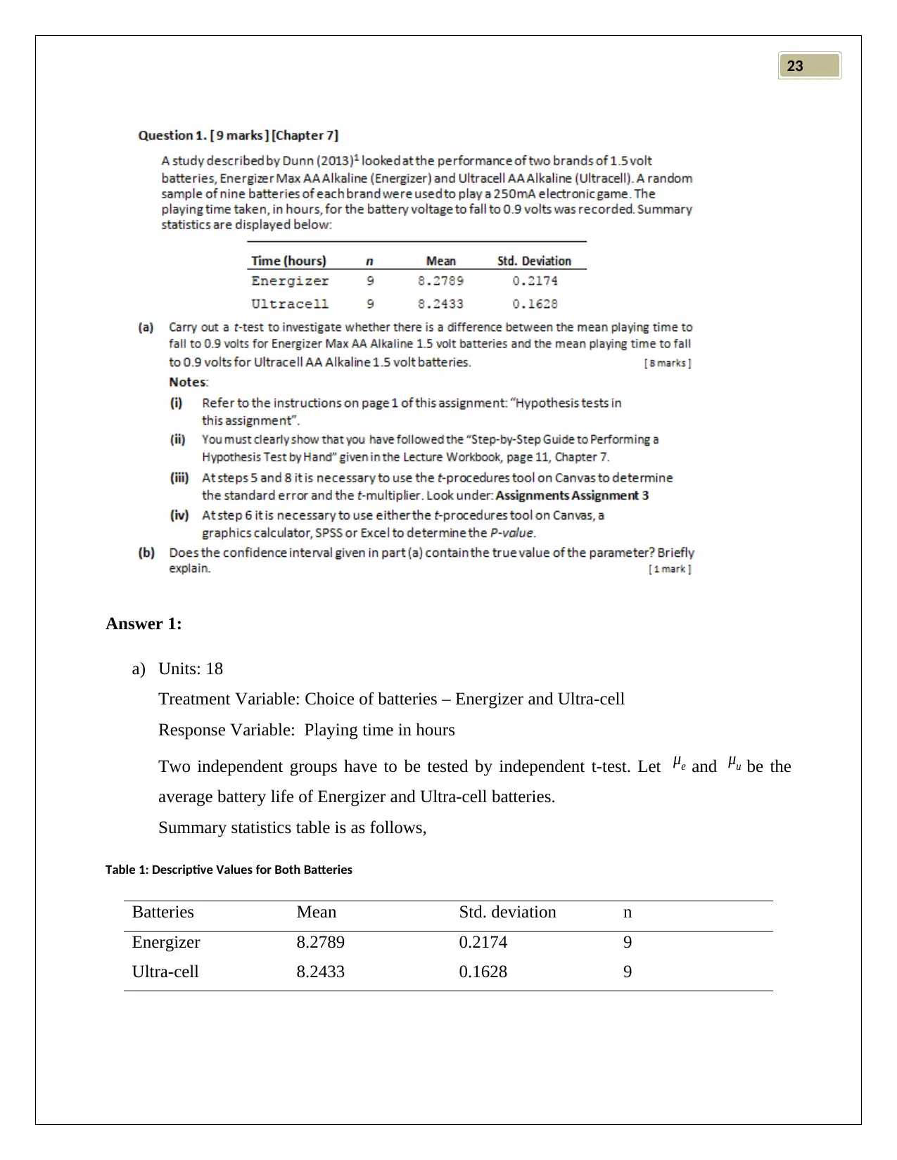
Answer 1:
a) Units: 18
Treatment Variable: Choice of batteries – Energizer and Ultra-cell
Response Variable: Playing time in hours
Two independent groups have to be tested by independent t-test. Let μe and μu be the
average battery life of Energizer and Ultra-cell batteries.
Summary statistics table is as follows,
Table 1: Descriptive Values for Both Batteries
Batteries Mean Std. deviation n
Energizer 8.2789 0.2174 9
Ultra-cell 8.2433 0.1628 9

23
Independent t-test
1. μe - μu = the difference between average playing life time in hours of Energizer and
Ultra-cell batteries.
2. Null Hypothesis: H0: μe - μu =0
3. Alternate Hypothesis: H1: μe - μu ¿ 0 (two-tailed)
4. From summary statistics of the sample survey, xe
−
−xu
−
= 8.2789 - 8.2433 = 0.0356
5. S.E ( xe
−
−xu
−
) = 0.0905 (from t‐procedures tool on Canvas) and the test statistic was
calculated using the formula
t = estimate−hypothesised value
s tan dard error =0 . 3933 as
t= 0. 0356−0
0. 0905 =0 . 3933 with 9 degrees of freedom.
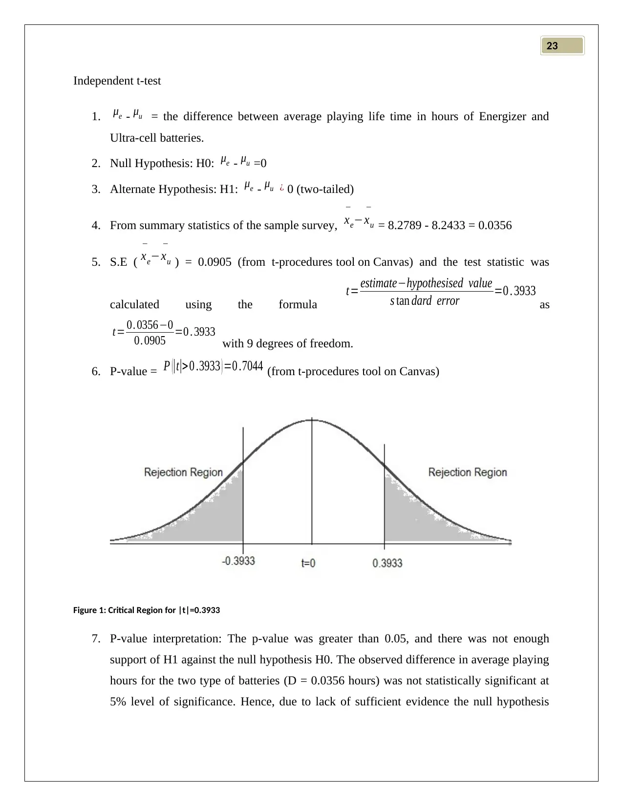
6. P-value = P (|t|> 0 .3933 ) =0 .7044 (from t‐procedures tool on Canvas)
Figure 1: Critical Region for |t|=0.3933
7. P-value interpretation: The p-value was greater than 0.05, and there was not enough
support of H1 against the null hypothesis H0. The observed difference in average playing
hours for the two type of batteries (D = 0.0356 hours) was not statistically significant at
5% level of significance. Hence, due to lack of sufficient evidence the null hypothesis

23
could not be rejected. Therefore, there was no statistically significant difference between
averages of playing time due to both the batteries (Hinton, 2014).
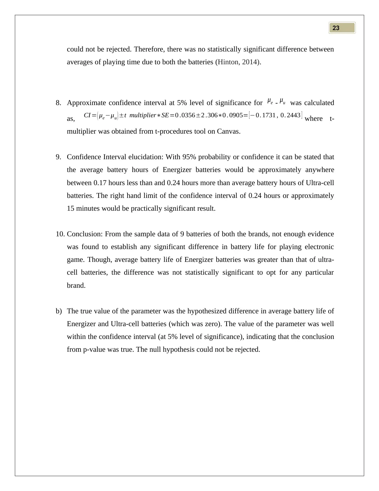
8. Approximate confidence interval at 5% level of significance for μe - μu was calculated
as, CI = ( μe −μu ) ±t multiplier∗SE=0 .0356±2 .306∗0 . 0905= [−0. 1731 , 0. 2443 ] where t-
multiplier was obtained from t‐procedures tool on Canvas.
9. Confidence Interval elucidation: With 95% probability or confidence it can be stated that
the average battery hours of Energizer batteries would be approximately anywhere
between 0.17 hours less than and 0.24 hours more than average battery hours of Ultra-cell
batteries. The right hand limit of the confidence interval of 0.24 hours or approximately
15 minutes would be practically significant result.
10. Conclusion: From the sample data of 9 batteries of both the brands, not enough evidence
was found to establish any significant difference in battery life for playing electronic
game. Though, average battery life of Energizer batteries was greater than that of ultra-
cell batteries, the difference was not statistically significant to opt for any particular
brand.
b) The true value of the parameter was the hypothesized difference in average battery life of
Energizer and Ultra-cell batteries (which was zero). The value of the parameter was well
within the confidence interval (at 5% level of significance), indicating that the conclusion
from p-value was true. The null hypothesis could not be rejected.

23
Answer 2
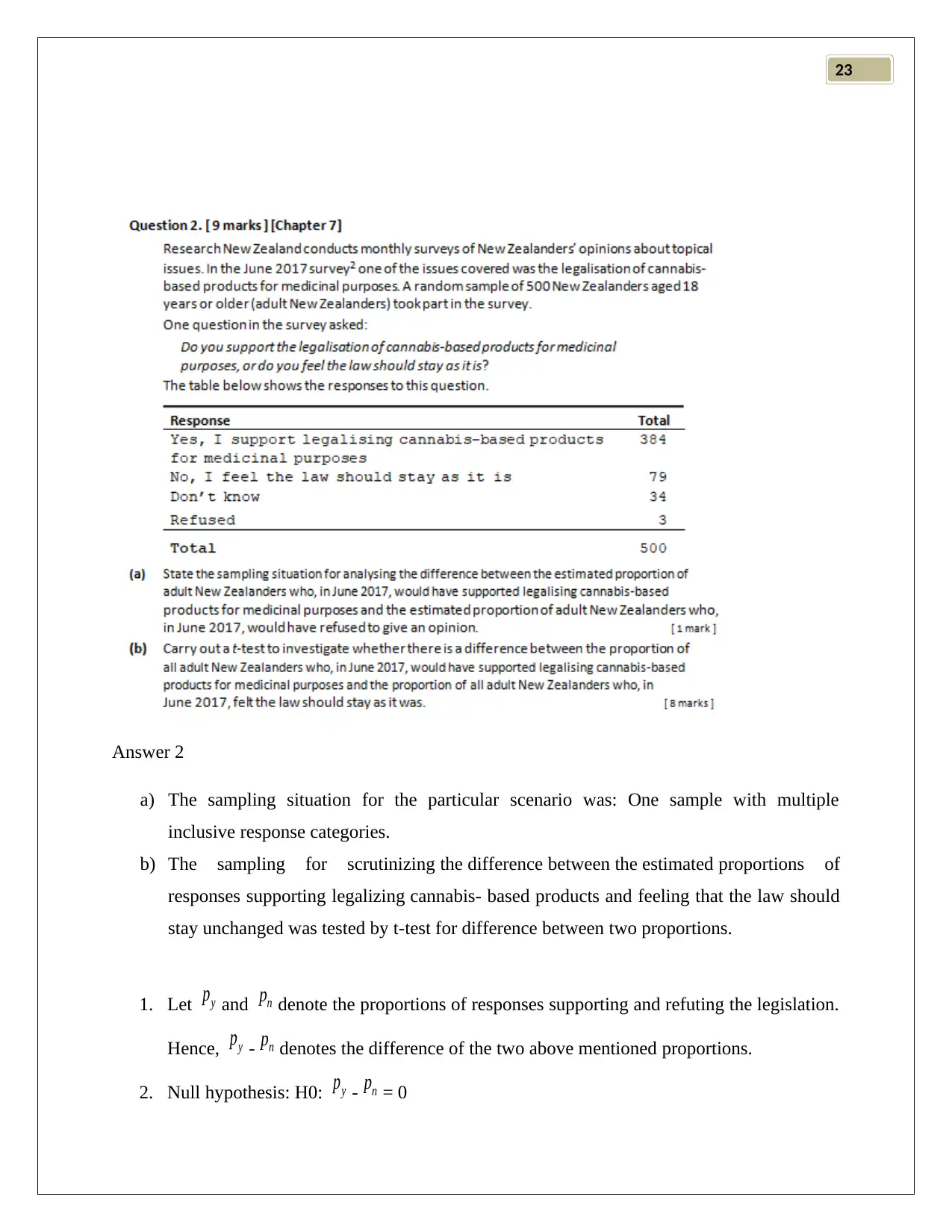
a) The sampling situation for the particular scenario was: One sample with multiple
inclusive response categories.
b) The sampling for scrutinizing the difference between the estimated proportions of
responses supporting legalizing cannabis- based products and feeling that the law should
stay unchanged was tested by t-test for difference between two proportions.
1. Let py and pn denote the proportions of responses supporting and refuting the legislation.
Hence, py - pn denotes the difference of the two above mentioned proportions.
2. Null hypothesis: H0: py - pn = 0

23
3. Alternate hypothesis: H1: py - pn ¿ 0 (two tailed)
4. Estimated difference: py
^¿
¿ - pn
^¿
¿ =
384
500 −79
500 =0 .61
5. The test statistic formula used
t = estimated difference−hypothesized difference
s tan dard error
For estimated difference = 0.61 and hypothesized difference = 0, the value of the standard
error was calculated using t‐procedures tool on Canvas as S.E ( py
^¿
¿ - pn
^¿
¿ ) = 0.0333 at 5%
level of significance. So the test statistic was calculated as
t = 0. 61−0
0 . 0333 =18 .3183 with
degrees of freedom = ∞
6. P-value = P (|t|> 18. 3183 ) =0. 0000 (from t‐procedures tool on Canvas)
Figure 2: Rejection Region for |t|=18.3183
7. Interpretation of p-value:
The p-value was greater than 0.05 at 5% level of significance and there was enough
evidence in favor of the alternate hypothesis against the null hypothesis. Hence, at 5%
level of significance, evidences from the difference in proportions of
adult New Zealanders in support and against the legislation of cannabis‐based products
usage for medicinal purposes were sufficient to reject the null hypothesis.

23
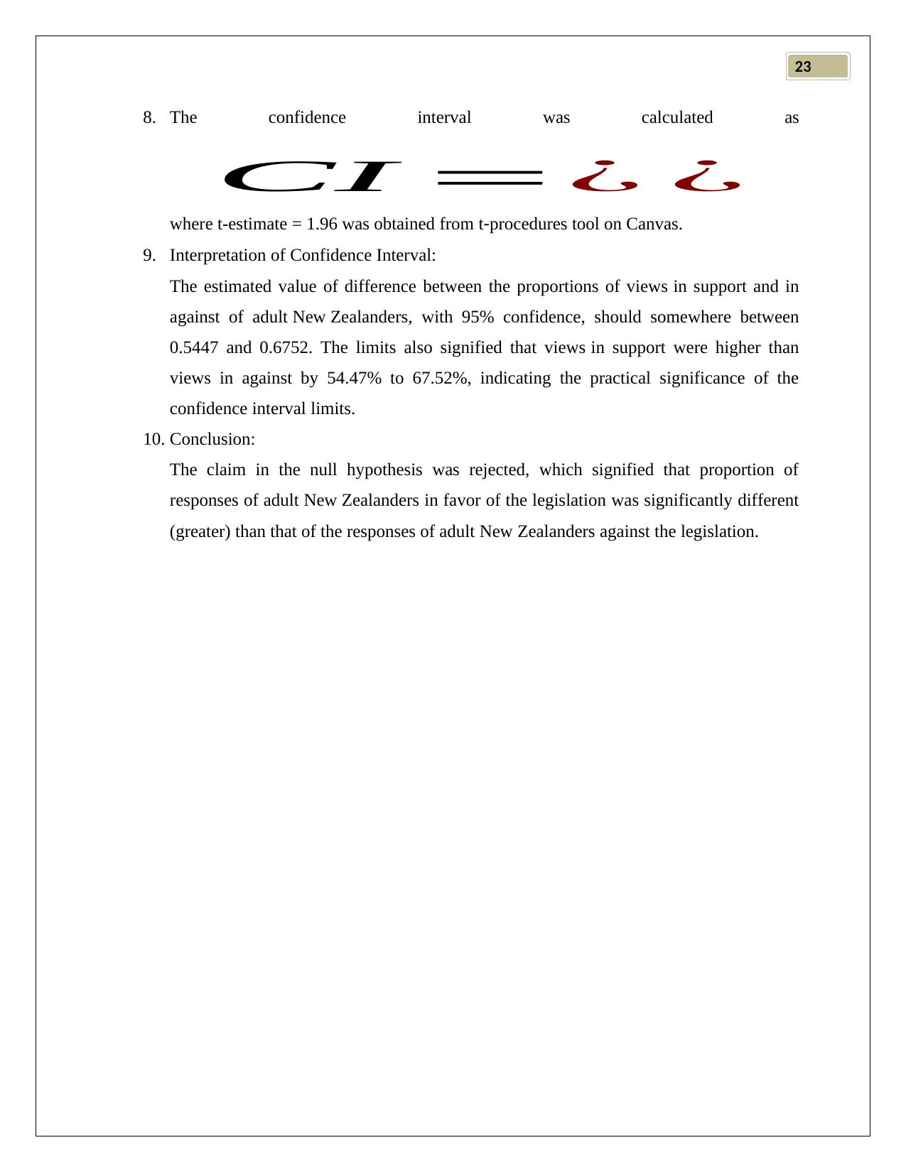
8. The confidence interval was calculated as
CI =¿ ¿
where t-estimate = 1.96 was obtained from t‐procedures tool on Canvas.
9. Interpretation of Confidence Interval:
The estimated value of difference between the proportions of views in support and in
against of adult New Zealanders, with 95% confidence, should somewhere between
0.5447 and 0.6752. The limits also signified that views in support were higher than
views in against by 54.47% to 67.52%, indicating the practical significance of the
confidence interval limits.
10. Conclusion:
The claim in the null hypothesis was rejected, which signified that proportion of
responses of adult New Zealanders in favor of the legislation was significantly different
(greater) than that of the responses of adult New Zealanders against the legislation.

23

23
Answer 3:
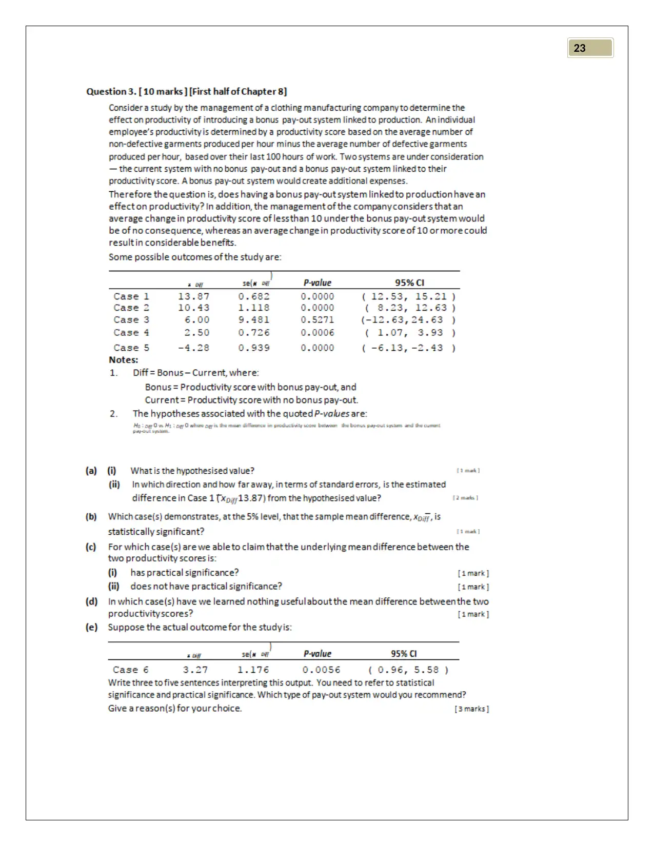
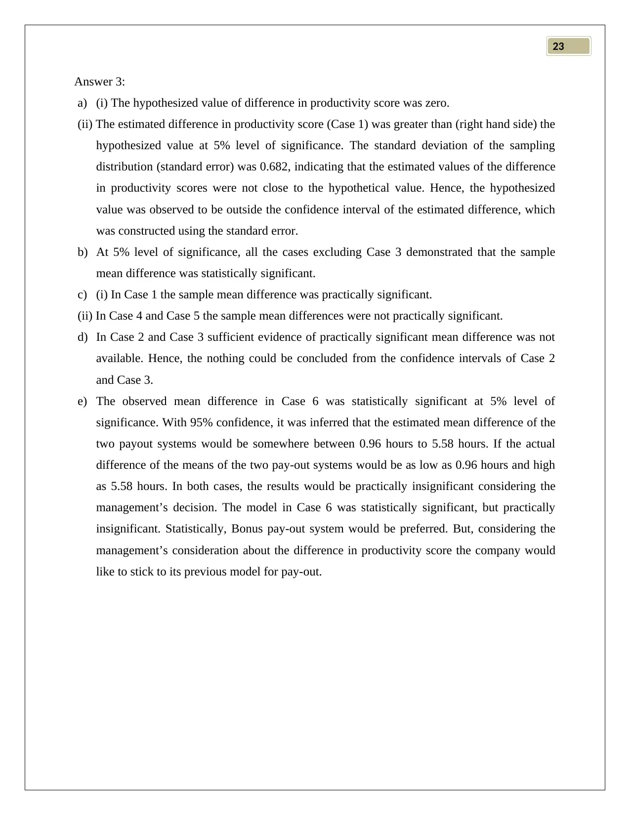
a) (i) The hypothesized value of difference in productivity score was zero.
(ii) The estimated difference in productivity score (Case 1) was greater than (right hand side) the
hypothesized value at 5% level of significance. The standard deviation of the sampling
distribution (standard error) was 0.682, indicating that the estimated values of the difference
in productivity scores were not close to the hypothetical value. Hence, the hypothesized
value was observed to be outside the confidence interval of the estimated difference, which
was constructed using the standard error.
b) At 5% level of significance, all the cases excluding Case 3 demonstrated that the sample
mean difference was statistically significant.
c) (i) In Case 1 the sample mean difference was practically significant.
(ii) In Case 4 and Case 5 the sample mean differences were not practically significant.
d) In Case 2 and Case 3 sufficient evidence of practically significant mean difference was not
available. Hence, the nothing could be concluded from the confidence intervals of Case 2
and Case 3.
e) The observed mean difference in Case 6 was statistically significant at 5% level of
significance. With 95% confidence, it was inferred that the estimated mean difference of the
two payout systems would be somewhere between 0.96 hours to 5.58 hours. If the actual
difference of the means of the two pay-out systems would be as low as 0.96 hours and high
as 5.58 hours. In both cases, the results would be practically insignificant considering the
management’s decision. The model in Case 6 was statistically significant, but practically
insignificant. Statistically, Bonus pay-out system would be preferred. But, considering the
management’s consideration about the difference in productivity score the company would
like to stick to its previous model for pay-out.

23
Answer 4
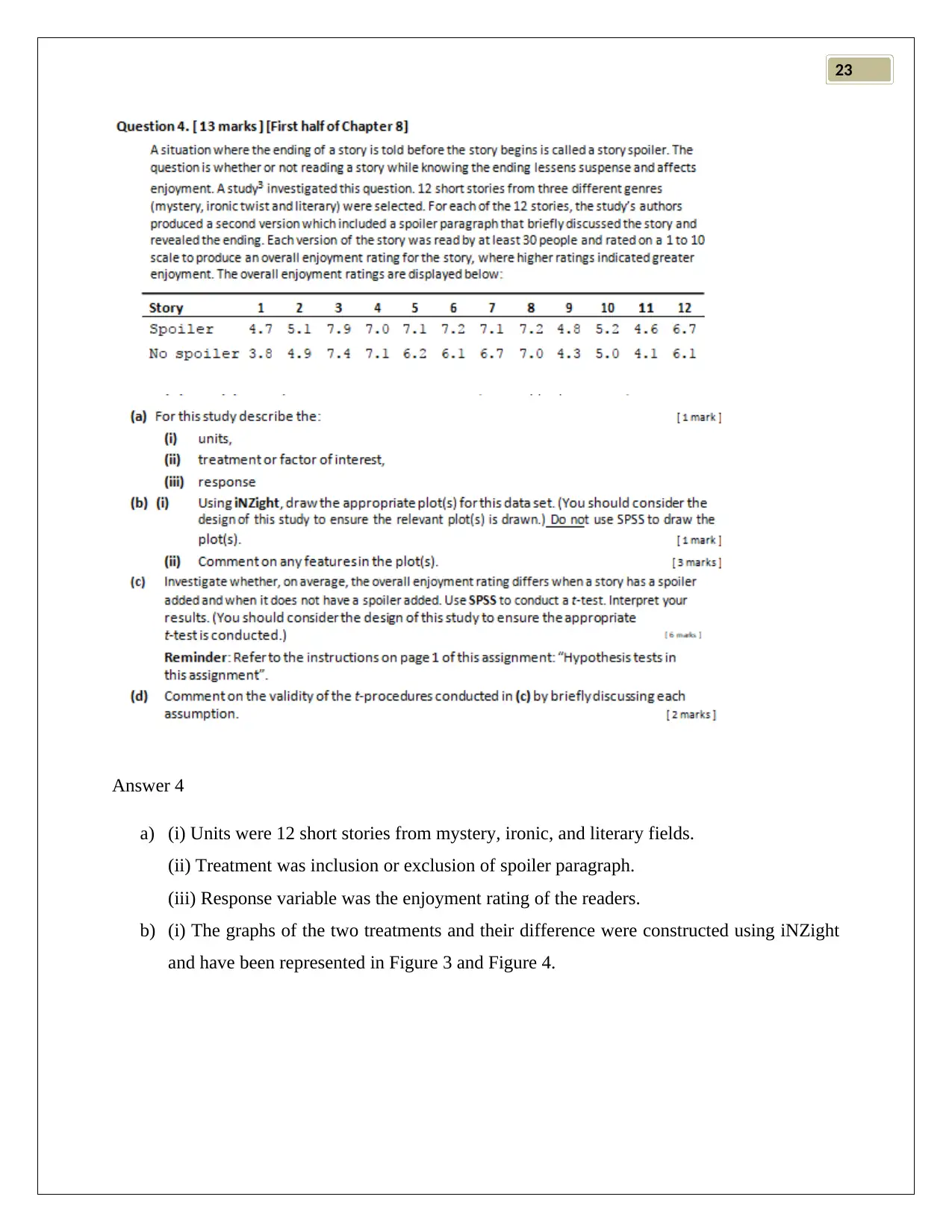
a) (i) Units were 12 short stories from mystery, ironic, and literary fields.
(ii) Treatment was inclusion or exclusion of spoiler paragraph.
(iii) Response variable was the enjoyment rating of the readers.
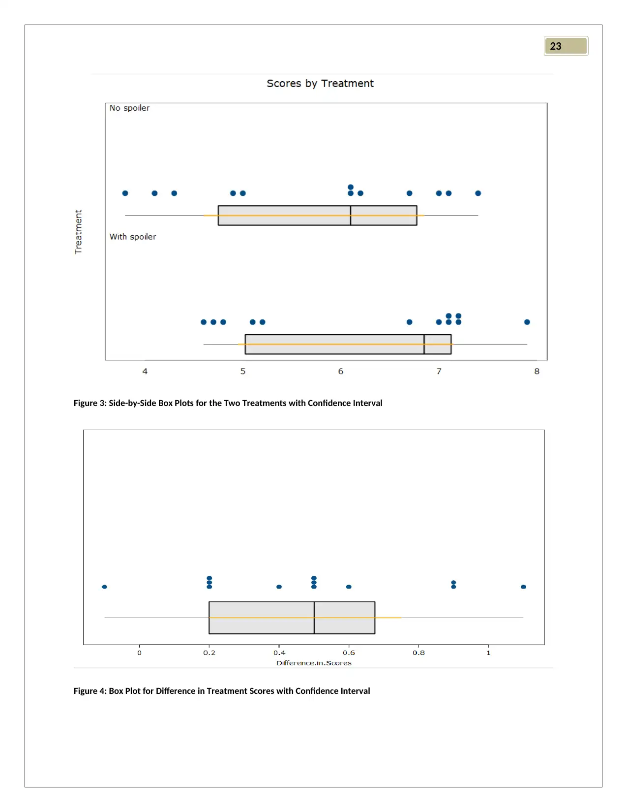
b) (i) The graphs of the two treatments and their difference were constructed using iNZight
and have been represented in Figure 3 and Figure 4.

23
Figure 3: Side-by-Side Box Plots for the Two Treatments with Confidence Interval
Figure 4: Box Plot for Difference in Treatment Scores with Confidence Interval

23
(ii) From Figure 3 side-by-side box plots, it was evident that median of enjoyment scores
of the stories was greater in case of spoiler paragraph in front of the story. The median
enjoyment score for stories with spoiler was nearly 7.0, whereas the median score of
enjoyment for the stories without spoiler paragraph was near the 6.0 mark. With spoiler
paragraph the distribution of enjoyment scores was highly left skewed compared to that
of the scores without spoiler paragraph.
The box plot of difference in the enjoyment scores were plotted and has been represented
in Figure 4. The median of difference in enjoyment scores was around 0.5, and the
distribution was observed to follow Gaussian distribution.
c) The difference between average enjoyment scores for the two treatments was verified by
t-test as follows.
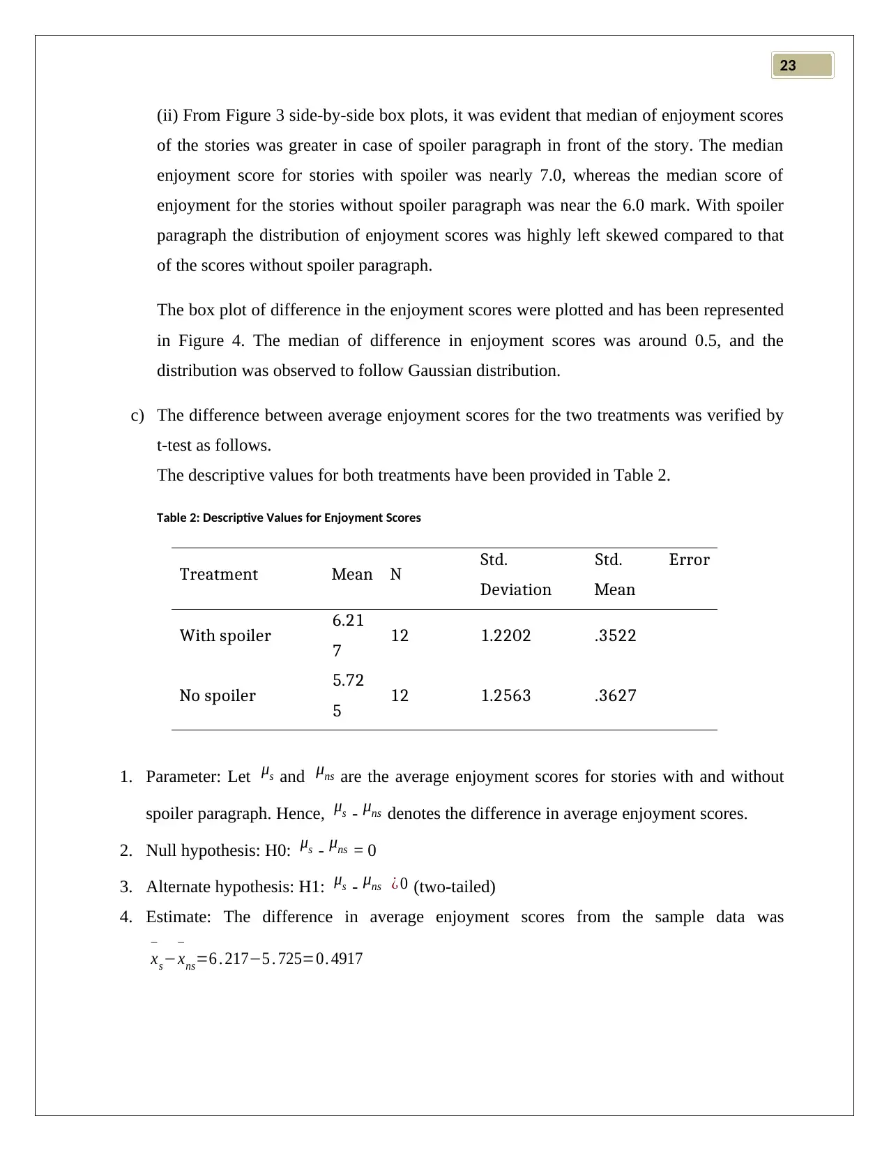
The descriptive values for both treatments have been provided in Table 2.
Table 2: Descriptive Values for Enjoyment Scores
Treatment Mean N Std.
Deviation
Std. Error
Mean
With spoiler 6.21
7 12 1.2202 .3522
No spoiler 5.72
5 12 1.2563 .3627
1. Parameter: Let μs and μns are the average enjoyment scores for stories with and without
spoiler paragraph. Hence, μs - μns denotes the difference in average enjoyment scores.
2. Null hypothesis: H0: μs - μns = 0
3. Alternate hypothesis: H1: μs - μns ¿ 0 (two-tailed)
4. Estimate: The difference in average enjoyment scores from the sample data was
x
−
s−x
−
ns=6 . 217−5 . 725=0. 4917