STATS 101/101G/108: Statistical Analysis, Hypothesis Testing 2018
VerifiedAdded on 2023/06/03
|10
|3831
|371
Homework Assignment
AI Summary
This assignment solution for STATS 101/101G/108 covers hypothesis testing, confidence intervals, and statistical significance. It includes problems involving t-tests to compare battery performance and opinions on cannabis legalization. The solution details the steps of hypothesis testing, including stating null and alternative hypotheses, determining significance levels, calculating test statistics, and interpreting p-values. It also addresses practical significance and the interpretation of confidence intervals in the context of a bonus payout system's effect on productivity. Further, the assignment examines the impact of story spoilers on enjoyment ratings, using appropriate plots and hypothesis testing to draw conclusions about the data. The document provides detailed calculations, SPSS outputs, and interpretations to guide students through the statistical analysis.
Running head: INTRODUCTION TO STATISTICS 1
STATS 101/101G/108 Introduction to Statistics
Assignment 3, Second Semester 2018
[Name]
[Date of Submission]
[Type here]
STATS 101/101G/108 Introduction to Statistics
Assignment 3, Second Semester 2018
[Name]
[Date of Submission]
[Type here]
Paraphrase This Document
Need a fresh take? Get an instant paraphrase of this document with our AI Paraphraser
INTRODUCTION TO STATISTICS 2
Question 1. [9 marks] [Chapter 7]
A study described by Dunn (2013) looked at the performance of two brands of 1.5 volt batteries, Energizer Max AA Alkaline
(Energizer) and Ultracell AA Alkaline (Ultracell). A random sample of nine batteries of each brand were used to play a 250mA
electronic game. The playing time taken, in hours, for the battery voltage to fall to 0.9 volts was recorded. Summary statistics are
displayed
below:
Time
(hours)
Energizer 9
Mean
8.2789
Std.
Deviation
0.2174
Ultracell 9 8.2433 0.1628
(a) Carry out a t‐test to investigate whether there is a difference between the mean playing time to fall to 0.9 volts for Energizer Max
AA Alkaline 1.5 volt batteries and the mean playing time to fall to 0.9 volts for Ultracell AA Alkaline 1.5 volt batteries.
[ 8 marks ]
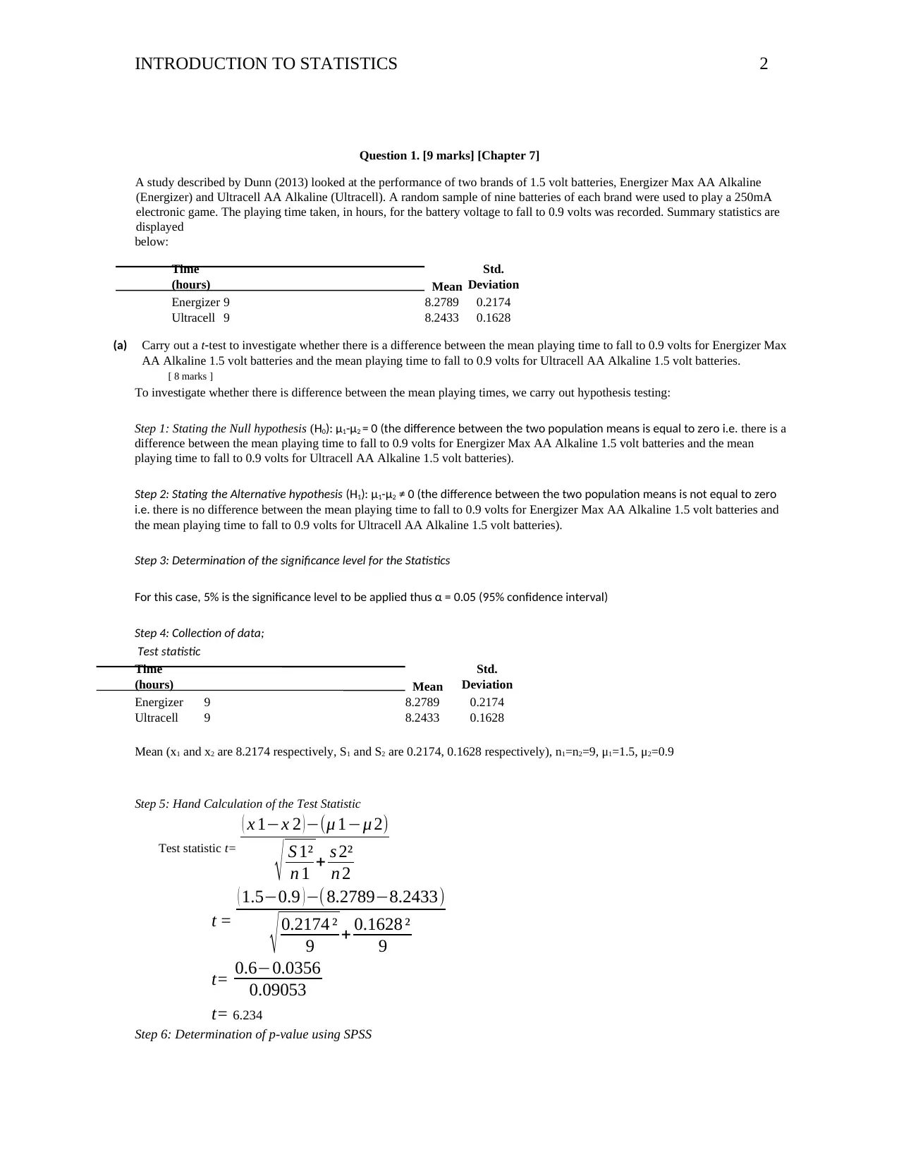
To investigate whether there is difference between the mean playing times, we carry out hypothesis testing:
Step 1: Stating the Null hypothesis (H0): μ1-μ2 = 0 (the difference between the two population means is equal to zero i.e. there is a
difference between the mean playing time to fall to 0.9 volts for Energizer Max AA Alkaline 1.5 volt batteries and the mean
playing time to fall to 0.9 volts for Ultracell AA Alkaline 1.5 volt batteries).
Step 2: Stating the Alternative hypothesis (H1): μ1-μ2 ≠ 0 (the difference between the two population means is not equal to zero
i.e. there is no difference between the mean playing time to fall to 0.9 volts for Energizer Max AA Alkaline 1.5 volt batteries and
the mean playing time to fall to 0.9 volts for Ultracell AA Alkaline 1.5 volt batteries).
Step 3: Determination of the significance level for the Statistics
For this case, 5% is the significance level to be applied thus α = 0.05 (95% confidence interval)
Step 4: Collection of data;
Test statistic
Time
(hours)
Energizer 9
Mean
8.2789
Std.
Deviation
0.2174
Ultracell 9 8.2433 0.1628
Mean (x1 and x2 are 8.2174 respectively, S1 and S2 are 0.2174, 0.1628 respectively), n1=n2=9, μ1=1.5, μ2=0.9
Step 5: Hand Calculation of the Test Statistic
Test statistic t=
( x 1−x 2 )−(μ 1−μ 2)
√ S 1²
n 1 + s 2²
n 2
t =
( 1.5−0.9 ) −( 8.2789−8.2433)
√ 0.2174 ²
9 + 0.1628 ²
9
t= 0.6−0.0356
0.09053
t= 6.234
Step 6: Determination of p-value using SPSS
Question 1. [9 marks] [Chapter 7]
A study described by Dunn (2013) looked at the performance of two brands of 1.5 volt batteries, Energizer Max AA Alkaline
(Energizer) and Ultracell AA Alkaline (Ultracell). A random sample of nine batteries of each brand were used to play a 250mA
electronic game. The playing time taken, in hours, for the battery voltage to fall to 0.9 volts was recorded. Summary statistics are
displayed
below:
Time
(hours)
Energizer 9
Mean
8.2789
Std.
Deviation
0.2174
Ultracell 9 8.2433 0.1628
(a) Carry out a t‐test to investigate whether there is a difference between the mean playing time to fall to 0.9 volts for Energizer Max
AA Alkaline 1.5 volt batteries and the mean playing time to fall to 0.9 volts for Ultracell AA Alkaline 1.5 volt batteries.
[ 8 marks ]
To investigate whether there is difference between the mean playing times, we carry out hypothesis testing:
Step 1: Stating the Null hypothesis (H0): μ1-μ2 = 0 (the difference between the two population means is equal to zero i.e. there is a
difference between the mean playing time to fall to 0.9 volts for Energizer Max AA Alkaline 1.5 volt batteries and the mean
playing time to fall to 0.9 volts for Ultracell AA Alkaline 1.5 volt batteries).
Step 2: Stating the Alternative hypothesis (H1): μ1-μ2 ≠ 0 (the difference between the two population means is not equal to zero
i.e. there is no difference between the mean playing time to fall to 0.9 volts for Energizer Max AA Alkaline 1.5 volt batteries and
the mean playing time to fall to 0.9 volts for Ultracell AA Alkaline 1.5 volt batteries).
Step 3: Determination of the significance level for the Statistics
For this case, 5% is the significance level to be applied thus α = 0.05 (95% confidence interval)
Step 4: Collection of data;
Test statistic
Time
(hours)
Energizer 9
Mean
8.2789
Std.
Deviation
0.2174
Ultracell 9 8.2433 0.1628
Mean (x1 and x2 are 8.2174 respectively, S1 and S2 are 0.2174, 0.1628 respectively), n1=n2=9, μ1=1.5, μ2=0.9
Step 5: Hand Calculation of the Test Statistic
Test statistic t=
( x 1−x 2 )−(μ 1−μ 2)
√ S 1²
n 1 + s 2²
n 2
t =
( 1.5−0.9 ) −( 8.2789−8.2433)
√ 0.2174 ²
9 + 0.1628 ²
9
t= 0.6−0.0356
0.09053
t= 6.234
Step 6: Determination of p-value using SPSS
INTRODUCTION TO STATISTICS 3
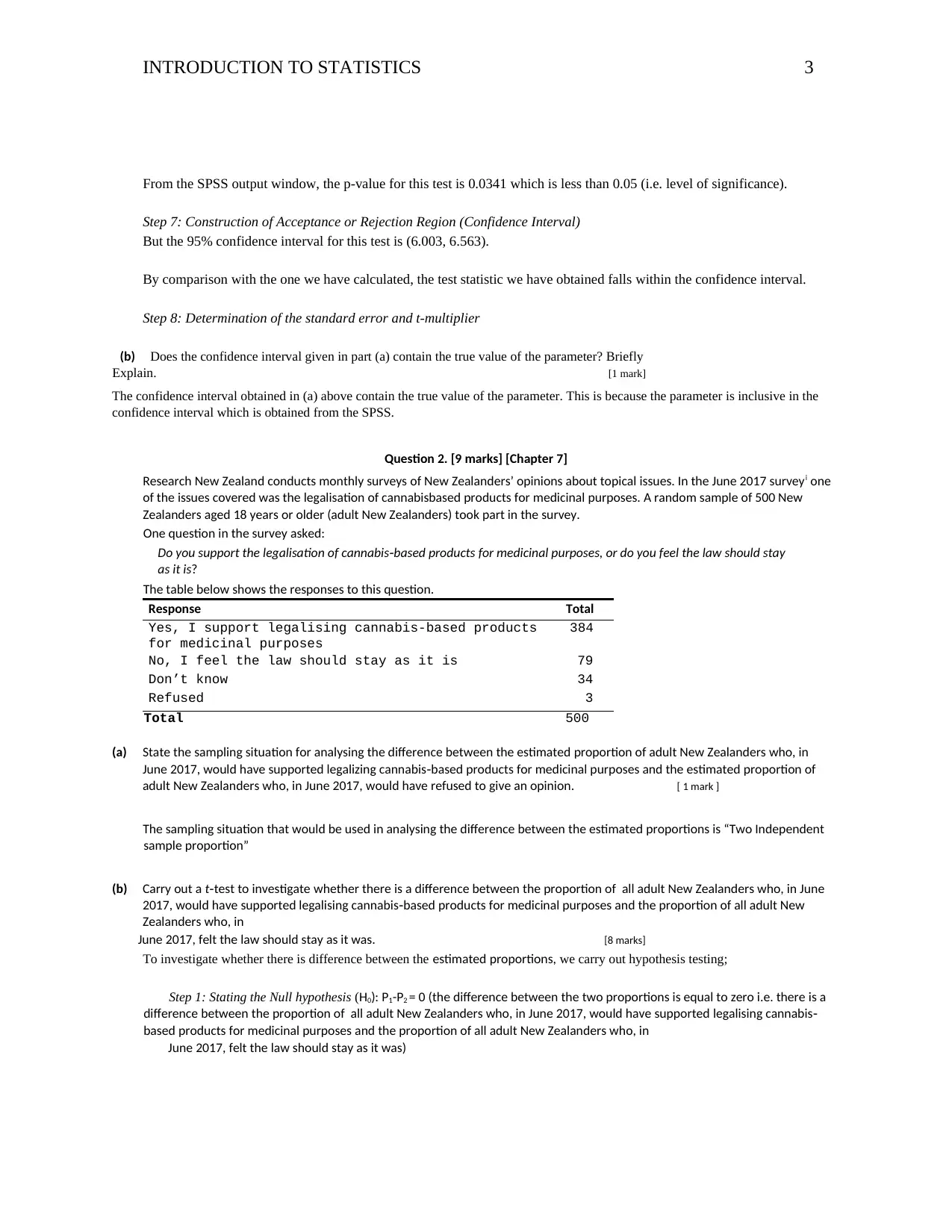
From the SPSS output window, the p-value for this test is 0.0341 which is less than 0.05 (i.e. level of significance).
Step 7: Construction of Acceptance or Rejection Region (Confidence Interval)
But the 95% confidence interval for this test is (6.003, 6.563).
By comparison with the one we have calculated, the test statistic we have obtained falls within the confidence interval.
Step 8: Determination of the standard error and t-multiplier
(b) Does the confidence interval given in part (a) contain the true value of the parameter? Briefly
Explain. [1 mark]
The confidence interval obtained in (a) above contain the true value of the parameter. This is because the parameter is inclusive in the
confidence interval which is obtained from the SPSS.
Question 2. [9 marks] [Chapter 7]
Research New Zealand conducts monthly surveys of New Zealanders’ opinions about topical issues. In the June 2017 surveyi one
of the issues covered was the legalisation of cannabisbased products for medicinal purposes. A random sample of 500 New
Zealanders aged 18 years or older (adult New Zealanders) took part in the survey.
One question in the survey asked:
Do you support the legalisation of cannabis based products for medicinal purposes, or do you feel the law should stay‐
as it is?
The table below shows the responses to this question.
Response Total
Yes, I support legalising cannabis-based products
for medicinal purposes
384
No, I feel the law should stay as it is 79
Don’t know 34
Refused 3
Total 500
(a) State the sampling situation for analysing the difference between the estimated proportion of adult New Zealanders who, in
June 2017, would have supported legalizing cannabis based products for medicinal purposes and the estimated proportion of‐
adult New Zealanders who, in June 2017, would have refused to give an opinion. [ 1 mark ]
The sampling situation that would be used in analysing the difference between the estimated proportions is “Two Independent
sample proportion”
(b) Carry out a t test to investigate whether there is a difference between the proportion of all adult New Zealanders who, in June‐
2017, would have supported legalising cannabis based products for medicinal purposes and the proportion of all adult New‐
Zealanders who, in
June 2017, felt the law should stay as it was. [8 marks]
To investigate whether there is difference between the estimated proportions, we carry out hypothesis testing;
Step 1: Stating the Null hypothesis (H0): P1-P2 = 0 (the difference between the two proportions is equal to zero i.e. there is a
difference between the proportion of all adult New Zealanders who, in June 2017, would have supported legalising cannabis‐
based products for medicinal purposes and the proportion of all adult New Zealanders who, in
June 2017, felt the law should stay as it was)
⊘ This is a preview!⊘
Do you want full access?
Subscribe today to unlock all pages.
Trusted by 1+ million students worldwide
INTRODUCTION TO STATISTICS 4
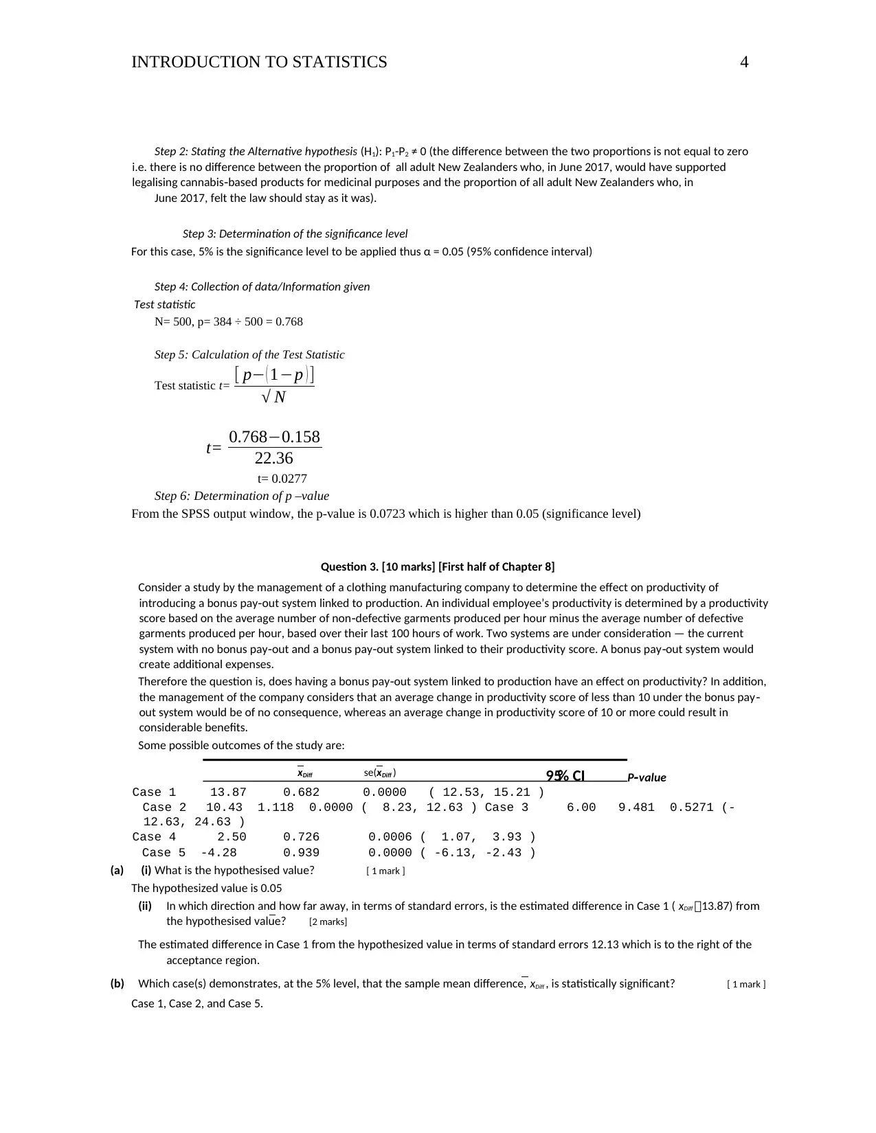
Step 2: Stating the Alternative hypothesis (H1): P1-P2 ≠ 0 (the difference between the two proportions is not equal to zero
i.e. there is no difference between the proportion of all adult New Zealanders who, in June 2017, would have supported
legalising cannabis based products for medicinal purposes and the proportion of all adult New Zealanders who, in‐
June 2017, felt the law should stay as it was).
Step 3: Determination of the significance level
For this case, 5% is the significance level to be applied thus α = 0.05 (95% confidence interval)
Step 4: Collection of data/Information given
Test statistic
N= 500, p= 384 ÷ 500 = 0.768
Step 5: Calculation of the Test Statistic
Test statistic t= [ p− ( 1−p ) ]
√ N
t= 0.768−0.158
22.36
t= 0.0277
Step 6: Determination of p –value
From the SPSS output window, the p-value is 0.0723 which is higher than 0.05 (significance level)
Question 3. [10 marks] [First half of Chapter 8]
Consider a study by the management of a clothing manufacturing company to determine the effect on productivity of
introducing a bonus pay out system linked to production. An individual employee’s productivity is determined by a productivity‐
score based on the average number of non defective garments produced per hour minus the average number of defective‐
garments produced per hour, based over their last 100 hours of work. Two systems are under consideration — the current
system with no bonus pay out and a bonus pay out system linked to their productivity score. A bonus pay out system would‐ ‐ ‐
create additional expenses.
Therefore the question is, does having a bonus pay out system linked to production have an effect on productivity? In addition,‐
the management of the company considers that an average change in productivity score of less than 10 under the bonus pay‐
out system would be of no consequence, whereas an average change in productivity score of 10 or more could result in
considerable benefits.
Some possible outcomes of the study are:
P value‐
Case 1 13.87 0.682 0.0000 ( 12.53, 15.21 )
Case 2 10.43 1.118 0.0000 ( 8.23, 12.63 ) Case 3 6.00 9.481 0.5271 (-
12.63, 24.63 )
Case 4 2.50 0.726 0.0006 ( 1.07, 3.93 )
Case 5 -4.28 0.939 0.0000 ( -6.13, -2.43 )
(a) (i) What is the hypothesised value? [ 1 mark ]
The hypothesized value is 0.05
(ii) In which direction and how far away, in terms of standard errors, is the estimated difference in Case 1 ( xDiff 13.87) from
the hypothesised value? [2 marks]
The estimated difference in Case 1 from the hypothesized value in terms of standard errors 12.13 which is to the right of the
acceptance region.
(b) Which case(s) demonstrates, at the 5% level, that the sample mean difference, xDiff , is statistically significant? [ 1 mark ]
Case 1, Case 2, and Case 5.
Diffx se( )Diffx 95% CI
Paraphrase This Document
Need a fresh take? Get an instant paraphrase of this document with our AI Paraphraser
x se ( )Diffx P value‐ 95% CI
0.0056
INTRODUCTION TO STATISTICS 5
(c) For which case(s) are we able to claim that the underlying mean difference between the two productivity scores is:
(i) Has practical significance? [ 1 mark ]
Case 1 and Case 4
(ii) Does not have practical significance? [ 1 mark ]
Case 5.
(d) In which case(s) have we learned nothing useful about the mean difference between the two
Productivity scores? [1 mark]
Case 2.
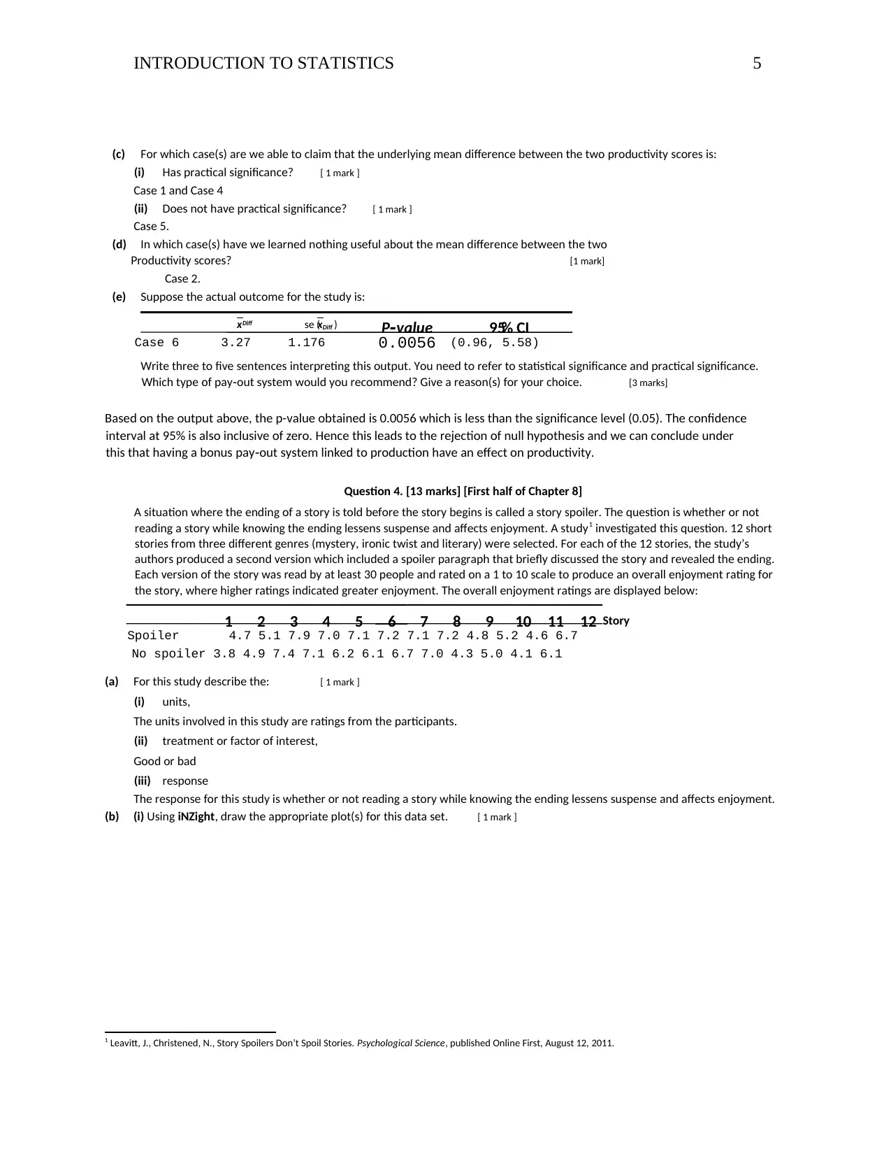
(e) Suppose the actual outcome for the study is:
Diff
Case 6 3.27 1.176 (0.96, 5.58)
Write three to five sentences interpreting this output. You need to refer to statistical significance and practical significance.
Which type of pay out system would you recommend? Give a reason(s) for your choice.‐ [3 marks]
Based on the output above, the p-value obtained is 0.0056 which is less than the significance level (0.05). The confidence
interval at 95% is also inclusive of zero. Hence this leads to the rejection of null hypothesis and we can conclude under
this that having a bonus pay out system linked to production have an effect on productivity.‐
Question 4. [13 marks] [First half of Chapter 8]
A situation where the ending of a story is told before the story begins is called a story spoiler. The question is whether or not
reading a story while knowing the ending lessens suspense and affects enjoyment. A study1 investigated this question. 12 short
stories from three different genres (mystery, ironic twist and literary) were selected. For each of the 12 stories, the study’s
authors produced a second version which included a spoiler paragraph that briefly discussed the story and revealed the ending.
Each version of the story was read by at least 30 people and rated on a 1 to 10 scale to produce an overall enjoyment rating for
the story, where higher ratings indicated greater enjoyment. The overall enjoyment ratings are displayed below:
Story
Spoiler 4.7 5.1 7.9 7.0 7.1 7.2 7.1 7.2 4.8 5.2 4.6 6.7
No spoiler 3.8 4.9 7.4 7.1 6.2 6.1 6.7 7.0 4.3 5.0 4.1 6.1
(a) For this study describe the: [ 1 mark ]
(i) units,
The units involved in this study are ratings from the participants.
(ii) treatment or factor of interest,
Good or bad
(iii) response
The response for this study is whether or not reading a story while knowing the ending lessens suspense and affects enjoyment.
(b) (i) Using iNZight, draw the appropriate plot(s) for this data set. [ 1 mark ]
1 Leavitt, J., Christened, N., Story Spoilers Don’t Spoil Stories. Psychological Science, published Online First, August 12, 2011.
1 2 3 4 5 6 7 8 9 10 11 12
0.0056
INTRODUCTION TO STATISTICS 5
(c) For which case(s) are we able to claim that the underlying mean difference between the two productivity scores is:
(i) Has practical significance? [ 1 mark ]
Case 1 and Case 4
(ii) Does not have practical significance? [ 1 mark ]
Case 5.
(d) In which case(s) have we learned nothing useful about the mean difference between the two
Productivity scores? [1 mark]
Case 2.
(e) Suppose the actual outcome for the study is:
Diff
Case 6 3.27 1.176 (0.96, 5.58)
Write three to five sentences interpreting this output. You need to refer to statistical significance and practical significance.
Which type of pay out system would you recommend? Give a reason(s) for your choice.‐ [3 marks]
Based on the output above, the p-value obtained is 0.0056 which is less than the significance level (0.05). The confidence
interval at 95% is also inclusive of zero. Hence this leads to the rejection of null hypothesis and we can conclude under
this that having a bonus pay out system linked to production have an effect on productivity.‐
Question 4. [13 marks] [First half of Chapter 8]
A situation where the ending of a story is told before the story begins is called a story spoiler. The question is whether or not
reading a story while knowing the ending lessens suspense and affects enjoyment. A study1 investigated this question. 12 short
stories from three different genres (mystery, ironic twist and literary) were selected. For each of the 12 stories, the study’s
authors produced a second version which included a spoiler paragraph that briefly discussed the story and revealed the ending.
Each version of the story was read by at least 30 people and rated on a 1 to 10 scale to produce an overall enjoyment rating for
the story, where higher ratings indicated greater enjoyment. The overall enjoyment ratings are displayed below:
Story
Spoiler 4.7 5.1 7.9 7.0 7.1 7.2 7.1 7.2 4.8 5.2 4.6 6.7
No spoiler 3.8 4.9 7.4 7.1 6.2 6.1 6.7 7.0 4.3 5.0 4.1 6.1
(a) For this study describe the: [ 1 mark ]
(i) units,
The units involved in this study are ratings from the participants.
(ii) treatment or factor of interest,
Good or bad
(iii) response
The response for this study is whether or not reading a story while knowing the ending lessens suspense and affects enjoyment.
(b) (i) Using iNZight, draw the appropriate plot(s) for this data set. [ 1 mark ]
1 Leavitt, J., Christened, N., Story Spoilers Don’t Spoil Stories. Psychological Science, published Online First, August 12, 2011.
1 2 3 4 5 6 7 8 9 10 11 12
INTRODUCTION TO STATISTICS 6
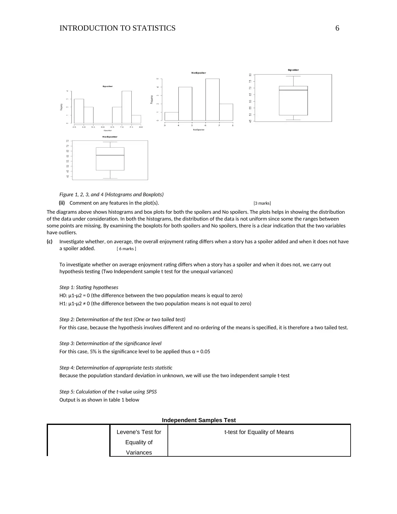
Figure 1, 2, 3, and 4 (Histograms and Boxplots)
(ii) Comment on any features in the plot(s). [3 marks]
The diagrams above shows histograms and box plots for both the spoilers and No spoilers. The plots helps in showing the distribution
of the data under consideration. In both the histograms, the distribution of the data is not uniform since some the ranges between
some points are missing. By examining the boxplots for both spoilers and No spoilers, there is a clear indication that the two variables
have outliers.
(c) Investigate whether, on average, the overall enjoyment rating differs when a story has a spoiler added and when it does not have
a spoiler added. [ 6 marks ]
To investigate whether on average enjoyment rating differs when a story has a spoiler and when it does not, we carry out
hypothesis testing (Two Independent sample t test for the unequal variances)
Step 1: Stating hypotheses
H0: μ1-μ2 = 0 (the difference between the two population means is equal to zero)
H1: μ1-μ2 ≠ 0 (the difference between the two population means is not equal to zero)
Step 2: Determination of the test (One or two tailed test)
For this case, because the hypothesis involves different and no ordering of the means is specified, it is therefore a two tailed test.
Step 3: Determination of the significance level
For this case, 5% is the significance level to be applied thus α = 0.05
Step 4: Determination of appropriate tests statistic
Because the population standard deviation in unknown, we will use the two independent sample t-test
Step 5: Calculation of the t-value using SPSS
Output is as shown in table 1 below
Independent Samples Test
Levene's Test for
Equality of
Variances
t-test for Equality of Means
⊘ This is a preview!⊘
Do you want full access?
Subscribe today to unlock all pages.
Trusted by 1+ million students worldwide
INTRODUCTION TO STATISTICS 7
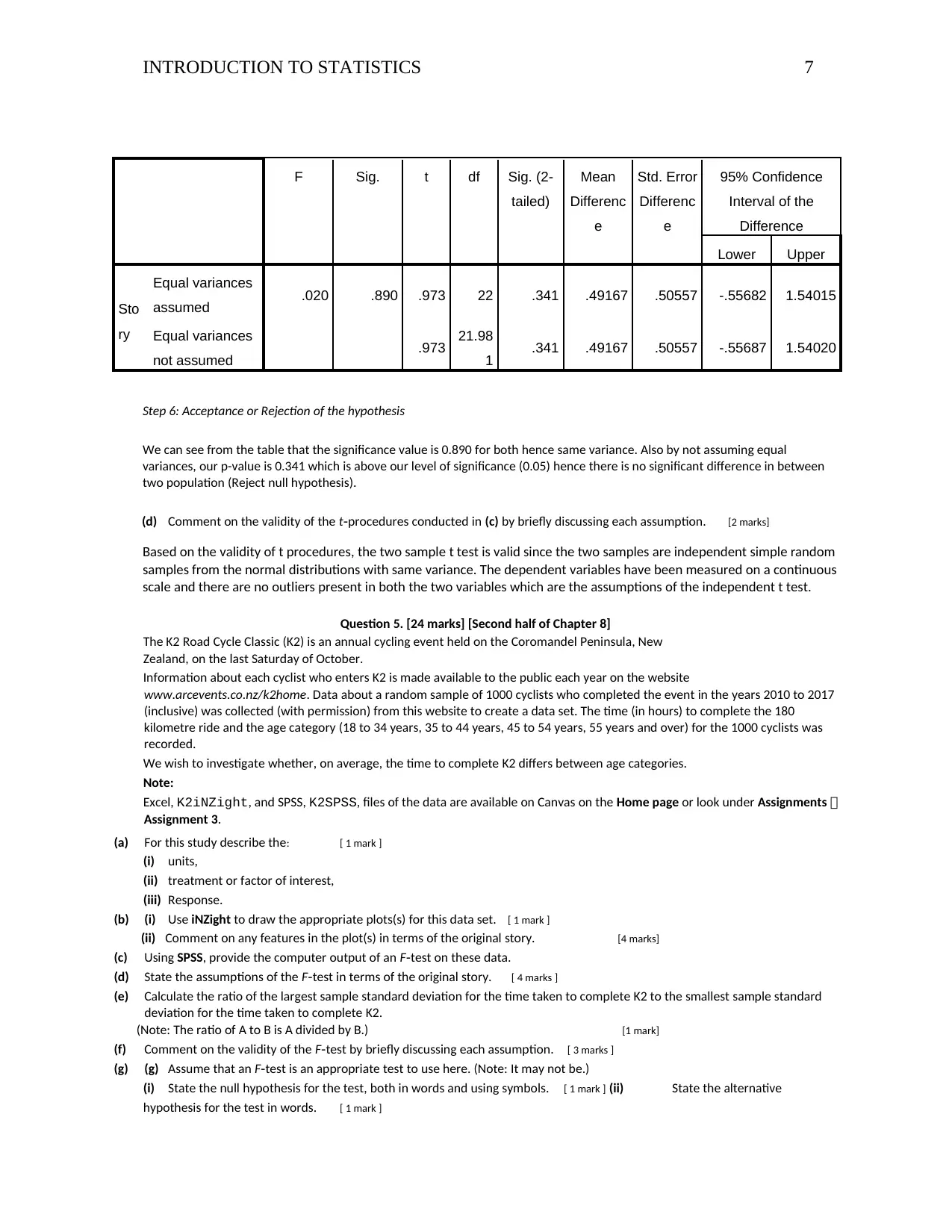
F Sig. t df Sig. (2-
tailed)
Mean
Differenc
e
Std. Error
Differenc
e
95% Confidence
Interval of the
Difference
Lower Upper
Sto
ry
Equal variances
assumed .020 .890 .973 22 .341 .49167 .50557 -.55682 1.54015
Equal variances
not assumed .973 21.98
1 .341 .49167 .50557 -.55687 1.54020
Step 6: Acceptance or Rejection of the hypothesis
We can see from the table that the significance value is 0.890 for both hence same variance. Also by not assuming equal
variances, our p-value is 0.341 which is above our level of significance (0.05) hence there is no significant difference in between
two population (Reject null hypothesis).
(d) Comment on the validity of the t procedures conducted in‐ (c) by briefly discussing each assumption. [2 marks]
Based on the validity of t procedures, the two sample t test is valid since the two samples are independent simple random
samples from the normal distributions with same variance. The dependent variables have been measured on a continuous
scale and there are no outliers present in both the two variables which are the assumptions of the independent t test.
Question 5. [24 marks] [Second half of Chapter 8]
The K2 Road Cycle Classic (K2) is an annual cycling event held on the Coromandel Peninsula, New
Zealand, on the last Saturday of October.
Information about each cyclist who enters K2 is made available to the public each year on the website
www.arcevents.co.nz/k2home. Data about a random sample of 1000 cyclists who completed the event in the years 2010 to 2017
(inclusive) was collected (with permission) from this website to create a data set. The time (in hours) to complete the 180
kilometre ride and the age category (18 to 34 years, 35 to 44 years, 45 to 54 years, 55 years and over) for the 1000 cyclists was
recorded.
We wish to investigate whether, on average, the time to complete K2 differs between age categories.
Note:
Excel, K2iNZight, and SPSS, K2SPSS, files of the data are available on Canvas on the Home page or look under Assignments
Assignment 3.
(a) For this study describe the: [ 1 mark ]
(i) units,
(ii) treatment or factor of interest,
(iii) Response.
(b) (i) Use iNZight to draw the appropriate plots(s) for this data set. [ 1 mark ]
(ii) Comment on any features in the plot(s) in terms of the original story. [4 marks]
(c) Using SPSS, provide the computer output of an F test on these data.‐
(d) State the assumptions of the F test in terms of the original story.‐ [ 4 marks ]
(e) Calculate the ratio of the largest sample standard deviation for the time taken to complete K2 to the smallest sample standard
deviation for the time taken to complete K2.
(Note: The ratio of A to B is A divided by B.) [1 mark]
(f) Comment on the validity of the F test by briefly discussing each assumption.‐ [ 3 marks ]
(g) (g) Assume that an F test is an appropriate test to use here. (Note: It may not be.)‐
(i) State the null hypothesis for the test, both in words and using symbols. [ 1 mark ] (ii) State the alternative
hypothesis for the test in words. [ 1 mark ]
Paraphrase This Document
Need a fresh take? Get an instant paraphrase of this document with our AI Paraphraser
INTRODUCTION TO STATISTICS 8
(iii) What does the result of the F test tell you about the underlying mean time taken to complete K2 for the four age‐
categories?
Explain your answer in 1 to 2 sentences. [1 mark]
(h) (i) Assume the Turkey’s pairwise comparisons are valid and appropriate. Investigate whether there is a difference between the
underlying mean time to complete K2 for cyclists aged 18 to 34 years and that for cyclists aged 35 to 44 years. Interpret the P‐
value and confidence interval.
[2 marks]
(ii) Between which pair (or pairs) of age categories were there significant differences
(at the 5% level) in the underlying mean time to complete K2? [1 mark]
(iii) Are we able to determine which age category has the slowest (i.e., highest) underlying mean time to complete K2? If so,
name the age category. [1 mark]
In three to five sentences, provide an overall conclusion for this study. [3 marks]
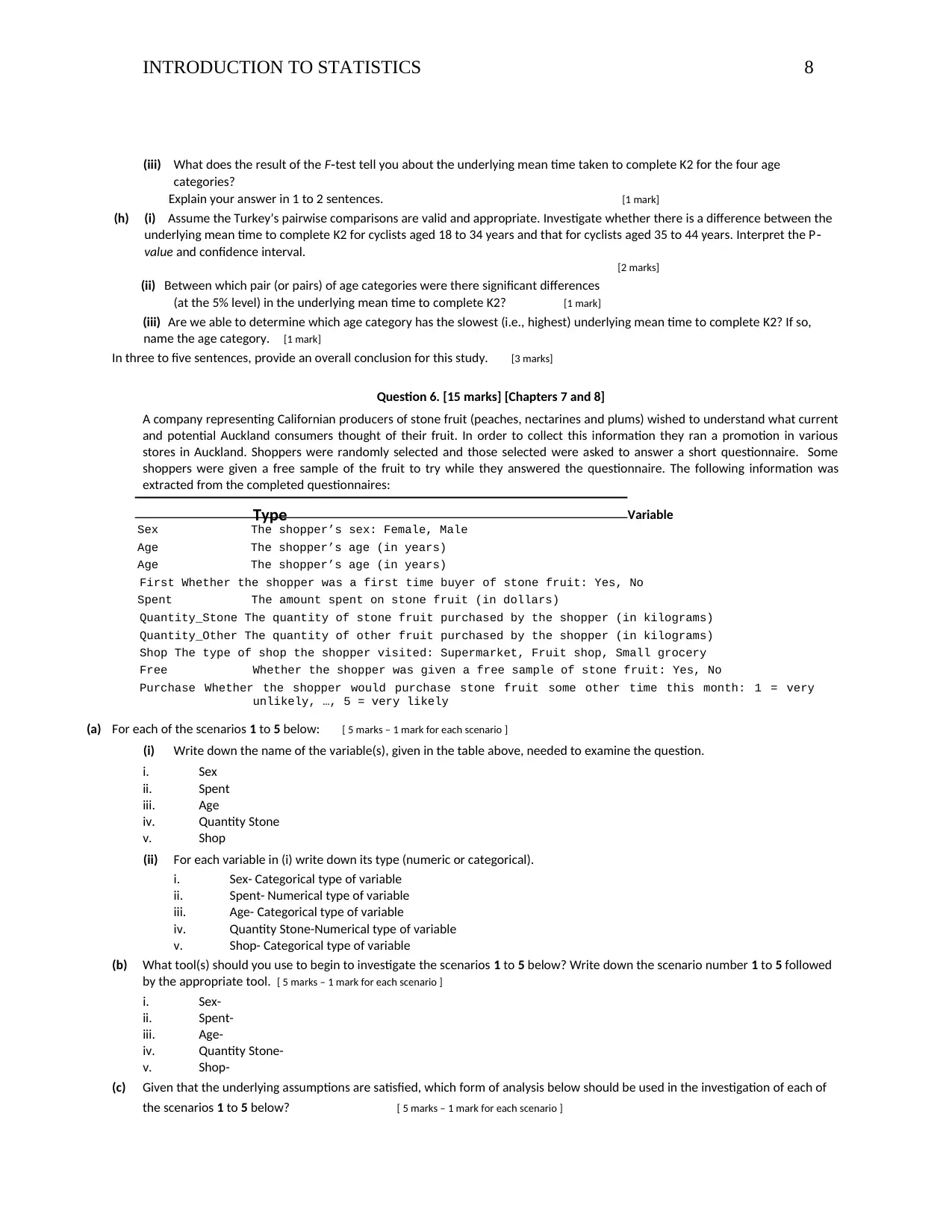
Question 6. [15 marks] [Chapters 7 and 8]
A company representing Californian producers of stone fruit (peaches, nectarines and plums) wished to understand what current
and potential Auckland consumers thought of their fruit. In order to collect this information they ran a promotion in various
stores in Auckland. Shoppers were randomly selected and those selected were asked to answer a short questionnaire. Some
shoppers were given a free sample of the fruit to try while they answered the questionnaire. The following information was
extracted from the completed questionnaires:
Variable
Sex The shopper’s sex: Female, Male
Age The shopper’s age (in years)
Age The shopper’s age (in years)
First Whether the shopper was a first time buyer of stone fruit: Yes, No
Spent The amount spent on stone fruit (in dollars)
Quantity_Stone The quantity of stone fruit purchased by the shopper (in kilograms)
Quantity_Other The quantity of other fruit purchased by the shopper (in kilograms)
Shop The type of shop the shopper visited: Supermarket, Fruit shop, Small grocery
Free Whether the shopper was given a free sample of stone fruit: Yes, No
Purchase Whether the shopper would purchase stone fruit some other time this month: 1 = very
unlikely, …, 5 = very likely
(a) For each of the scenarios 1 to 5 below: [ 5 marks – 1 mark for each scenario ]
(i) Write down the name of the variable(s), given in the table above, needed to examine the question.
i. Sex
ii. Spent
iii. Age
iv. Quantity Stone
v. Shop
(ii) For each variable in (i) write down its type (numeric or categorical).
i. Sex- Categorical type of variable
ii. Spent- Numerical type of variable
iii. Age- Categorical type of variable
iv. Quantity Stone-Numerical type of variable
v. Shop- Categorical type of variable
(b) What tool(s) should you use to begin to investigate the scenarios 1 to 5 below? Write down the scenario number 1 to 5 followed
by the appropriate tool. [ 5 marks – 1 mark for each scenario ]
i. Sex-
ii. Spent-
iii. Age-
iv. Quantity Stone-
v. Shop-
(c) Given that the underlying assumptions are satisfied, which form of analysis below should be used in the investigation of each of
the scenarios 1 to 5 below? [ 5 marks – 1 mark for each scenario ]
Type
(iii) What does the result of the F test tell you about the underlying mean time taken to complete K2 for the four age‐
categories?
Explain your answer in 1 to 2 sentences. [1 mark]
(h) (i) Assume the Turkey’s pairwise comparisons are valid and appropriate. Investigate whether there is a difference between the
underlying mean time to complete K2 for cyclists aged 18 to 34 years and that for cyclists aged 35 to 44 years. Interpret the P‐
value and confidence interval.
[2 marks]
(ii) Between which pair (or pairs) of age categories were there significant differences
(at the 5% level) in the underlying mean time to complete K2? [1 mark]
(iii) Are we able to determine which age category has the slowest (i.e., highest) underlying mean time to complete K2? If so,
name the age category. [1 mark]
In three to five sentences, provide an overall conclusion for this study. [3 marks]
Question 6. [15 marks] [Chapters 7 and 8]
A company representing Californian producers of stone fruit (peaches, nectarines and plums) wished to understand what current
and potential Auckland consumers thought of their fruit. In order to collect this information they ran a promotion in various
stores in Auckland. Shoppers were randomly selected and those selected were asked to answer a short questionnaire. Some
shoppers were given a free sample of the fruit to try while they answered the questionnaire. The following information was
extracted from the completed questionnaires:
Variable
Sex The shopper’s sex: Female, Male
Age The shopper’s age (in years)
Age The shopper’s age (in years)
First Whether the shopper was a first time buyer of stone fruit: Yes, No
Spent The amount spent on stone fruit (in dollars)
Quantity_Stone The quantity of stone fruit purchased by the shopper (in kilograms)
Quantity_Other The quantity of other fruit purchased by the shopper (in kilograms)
Shop The type of shop the shopper visited: Supermarket, Fruit shop, Small grocery
Free Whether the shopper was given a free sample of stone fruit: Yes, No
Purchase Whether the shopper would purchase stone fruit some other time this month: 1 = very
unlikely, …, 5 = very likely
(a) For each of the scenarios 1 to 5 below: [ 5 marks – 1 mark for each scenario ]
(i) Write down the name of the variable(s), given in the table above, needed to examine the question.
i. Sex
ii. Spent
iii. Age
iv. Quantity Stone
v. Shop
(ii) For each variable in (i) write down its type (numeric or categorical).
i. Sex- Categorical type of variable
ii. Spent- Numerical type of variable
iii. Age- Categorical type of variable
iv. Quantity Stone-Numerical type of variable
v. Shop- Categorical type of variable
(b) What tool(s) should you use to begin to investigate the scenarios 1 to 5 below? Write down the scenario number 1 to 5 followed
by the appropriate tool. [ 5 marks – 1 mark for each scenario ]
i. Sex-
ii. Spent-
iii. Age-
iv. Quantity Stone-
v. Shop-
(c) Given that the underlying assumptions are satisfied, which form of analysis below should be used in the investigation of each of
the scenarios 1 to 5 below? [ 5 marks – 1 mark for each scenario ]
Type

INTRODUCTION TO STATISTICS 9
i. Sex - D
ii. Spent- C
iii. Age- A
iv. Quantity Stone - F
v. Shop- A
i. Sex - D
ii. Spent- C
iii. Age- A
iv. Quantity Stone - F
v. Shop- A
⊘ This is a preview!⊘
Do you want full access?
Subscribe today to unlock all pages.
Trusted by 1+ million students worldwide

i
1 out of 10


Your All-in-One AI-Powered Toolkit for Academic Success.
+13062052269
info@desklib.com
Available 24*7 on WhatsApp / Email
![[object Object]](/_next/static/media/star-bottom.7253800d.svg)
Unlock your academic potential
Copyright © 2020–2026 A2Z Services. All Rights Reserved. Developed and managed by ZUCOL.