Comprehensive Coursework: Statistics, Probability, Data Analysis
VerifiedAdded on 2023/06/15
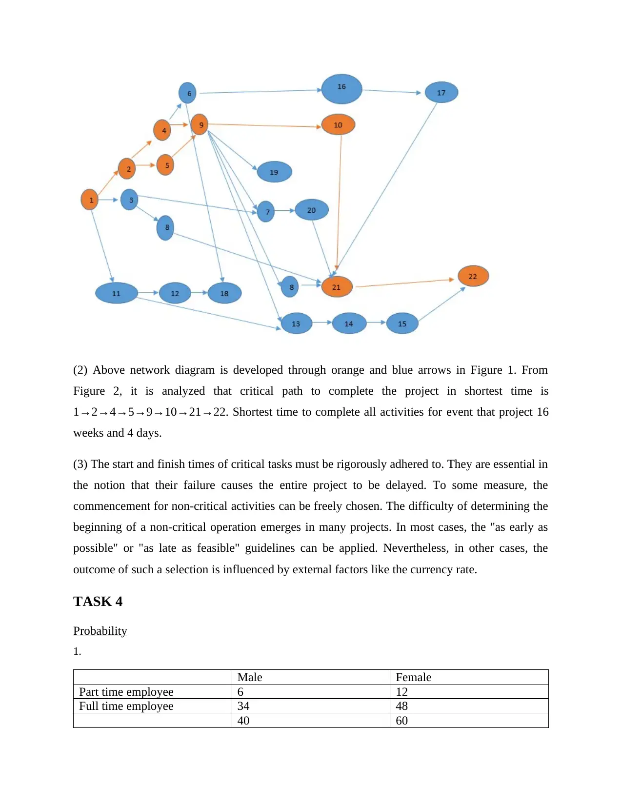
|11
|1473
|251
Homework Assignment
AI Summary
This coursework solution covers various statistical and probabilistic analyses. It includes descriptive statistics for grouped and ungrouped data, examining expenditures on a product. The coursework further delves into networking concepts, identifying critical paths, and analyzing probabilities related to employee demographics. Cost analysis, including break-even point determination, is performed. Finally, correlation and regression analyses are conducted to explore relationships between sales revenue, total costs, average order value, and net profit, providing insights into predictive modeling and variable dependencies. Desklib provides this and many more solved assignments.

Coursework 1 consists of
2 parts
2 parts
Paraphrase This Document
Need a fresh take? Get an instant paraphrase of this document with our AI Paraphraser

TABLE OF CONTENTS
TASK 1.......................................................................................................................................................3
Under grouped descriptive statics............................................................................................................3
TASK 2.......................................................................................................................................................3
Group Descriptive Statistics....................................................................................................................3
TASK 3.......................................................................................................................................................5
Networking..............................................................................................................................................5
TASK 4.......................................................................................................................................................6
Probability...............................................................................................................................................6
TASK 5.......................................................................................................................................................7
Costs and Break even..............................................................................................................................7
PART 2........................................................................................................................................................8
Relationship.............................................................................................................................................8

TASK 1
Under grouped descriptive statics
Table 1
Expenditure (£) on Selfie
Ring Light
Mean 35
Standard Error 0.97
Median 33.00
Mode 32.00
Standard Deviation 40
Sample Variance 54.04
Kurtosis -1.03
Skewness 0.33
Range 25.00
Minimum 24.00
Maximum 49.00
Sum 2030
Count 58
Interpretation: As per the above scenario it has been determined that different price is given by
the people for LED selfie ring light. To analysis the expenditure in detained manner require to
calculate mean and standard deviation that helps to know overall estimation. Mean is 35 and
standard deviation 40 after implementation effective methods for calculations.
TASK 2
Group Descriptive Statistics
1.
Table 2A
Expenditure (£) Frequency
Percentage
Frequency
⊘ This is a preview!⊘
Do you want full access?
Subscribe today to unlock all pages.

Trusted by 1+ million students worldwide

Under 25 2 8
25 and under 30 14 50
30 and under 35 16 50
35 and under 40 8 21
40 and under 45 11 26
45 and under 50 7 16
Total: 58 171
Table 2B
Expenditure (£)
Cumulative
Frequency
Cumulative
Percentage
Frequency
Less than 25 25 11
Less than 30 65 28
Less than 35 100 43
Less than 40 140 60
Less than 45 185 79
Less than 50 235 100
Table 2C
Expenditure
(£)
Frequency
(f)
Midpoint
(x) fx
(x-
mean) (x-mean)2 f(x-mean)2
Under 25 2 22.50 45 12.83 164.61 329.22
25 and under 30 14 27.50 385 17.83 317.91 4450.72
30 and under 35 16 32.50 520 22.83 521.21 8339.34
35 and under 40 8 37.50 300 27.83 774.51 6196.07
40 and under 45 11 42.50 467.5 32.83 1077.81 11855.90
45 and under 50 7 47.50 332.5 37.83 1431.11 10017.76
Total: 58
Paraphrase This Document
Need a fresh take? Get an instant paraphrase of this document with our AI Paraphraser

2.
Report 1: The advantage of producing table 2A, it helps to know actual percentage of expenses
which are paying by the customer in regard of product. It helps to analysis to profitability as
compare of expenses.
Report 2: As a measurement of frequency and percentage, the major benefit of cumulative
percentage above cumulative frequency is that it makes it possible to evaluate sets of
information. The only difference between the probability and cumulative percentage diagrams is
the vertical axis scale.
Report 3: Mean vale and standard deviation are different in task 1 and 2 and task 1 is more
accurate because it is calculating on basis of particular numbers.
3.
With reference to the figure, it is clearly visible that the minimum amount of the consumer need
for spending on the selfie ring light to belong to top 25% in terms of expenditure is till 5 % of the
expenditure. This is pertaining to the fact that below 25 there are less people.
TASK 3
Networking

(2) Above network diagram is developed through orange and blue arrows in Figure 1. From
Figure 2, it is analyzed that critical path to complete the project in shortest time is
1→2→4→5→9→10→21→22. Shortest time to complete all activities for event that project 16
weeks and 4 days.
(3) The start and finish times of critical tasks must be rigorously adhered to. They are essential in
the notion that their failure causes the entire project to be delayed. To some measure, the
commencement for non-critical activities can be freely chosen. The difficulty of determining the
beginning of a non-critical operation emerges in many projects. In most cases, the "as early as
possible" or "as late as feasible" guidelines can be applied. Nevertheless, in other cases, the
outcome of such a selection is influenced by external factors like the currency rate.
TASK 4
Probability
1.
Male Female
Part time employee 6 12
Full time employee 34 48
40 60
⊘ This is a preview!⊘
Do you want full access?
Subscribe today to unlock all pages.

Trusted by 1+ million students worldwide

2.
The probability of choosing male and working full time is as follows-
40/ 100 * 34/ 40
= 34/100
= 0.34
This implies that there is 0.34 chance that on selecting randomly the male who is working full
time will be selected.
TASK 5
Costs and Break even
Variable cost
High low method
Highest activity cost – lowest activity cost / Highest activity unit -Lowest
activity units
7
Highest activity
cost 360000
Highest activity
unit 42000
Lowest activity
cost 150000
Lowest activity
unit 12000
Fixed cost
Fixed cost Highest activity cost - (variable cost per unit* Highest activity units)
66000
Variable cost per unit 7
Highest activity cost 360000
Highest activity unit 42000
Paraphrase This Document
Need a fresh take? Get an instant paraphrase of this document with our AI Paraphraser

Lowest activity cost 150000
Lowest activity unit 12000
BEP
Particulars Formula Amount
selling price per unit 10
less: VC per unit 7
Contribution Selling price- VC 3
FC 66000
BEP (units) Fixed cost/ contribution 22000
BEP (rupees) 220000
With the analysis of the calculation it is clear that the BEP production units for company
is 22000. This implies that in case the production is 22000 units then the company will be in no
profit no loss situation. Once the company will start producing beyond this level then the
company will start earning profits.
PART 2
Relationship
Coefficient matrix
Sales
Revenu
e
(£'000)
Total
Costs
(£'000)
Averag
e
Order
Value
(£)
Net
Profit
(£'000)
Sales Revenue (£'000) 1
Total Costs (£'000) 0.8715 1
Average Order Value
(£) 0.99762 0.8738 1
Net Profit (£'000) 0.49984
0.0108
8
0.4909
3 1

2
With the help of above table, it can be seen that the best predictor of quarterly sales revenue is
average order value. This is pertaining to the fact that the correlation is maximum with this
predictor. Hence, it can be implied that best predictor is average order value.
3.
0 2 4 6 8 10 12
0
2
4
6
8
10
12
f(x) = NaN x + NaN
R² = 0 Sales Revenue (£'000)
4.
The correlation of coefficient states that the relation between the variables is very low that is
6.41 and this implies that the working of the sales revenue is not at all dependent over the
working of average order value.
5.
The regression equation is y= 6.4292x + 498.92
From this equation the gradient is 6.492 and the intercept is 498.92.
6.
When x = 100
Y= 6.4292 (100) + 498.92
⊘ This is a preview!⊘
Do you want full access?
Subscribe today to unlock all pages.

Trusted by 1+ million students worldwide

Y= 642.92 + 498.92
Y= 1141.84
7.
Introduction
The correlation is being referred to as the identification of the relation between two or
more variables. It is very important for the person that they must easily identify the relation
between the two variables.
With the help of the correlation matrix it is clear that there is high correlation of sales
with total cost and average order value but low with net profit. Further the total cost is very low
correlated with the net profit.
Moreover, the scatter plot diagram assisted in analysing the fact that there is fluctuating
trend within the profitability of the company. the reason underlying this fact is that in case the
sales revenue will not be in direction of increasing trend then this will be affecting the
profitability of the business.
In addition to this, the correlation matrix also highlighted the fact that the correlation
coefficient is low and this implies that changes within the independent factors will cause low
changes within the dependent factor.
Further with help of the regression it can be evaluated that whether there is any
significant relation being present in the two or more variables. Hence, the regression equation
created was y= 6.4292x + 498.92
The prediction with help of the regression equation evaluated that there is prediction of
1141.84 sales revenue for the next quarter. This prediction can be reliable because in the present
case the last profit is 691 and in case the product provided by company will be good then the
sales can be increased till 1141.84.
Conclusion
Paraphrase This Document
Need a fresh take? Get an instant paraphrase of this document with our AI Paraphraser

In the end it can be concluded that correlation is essential to be calculated as it highlights
the relation between the two or more variables. The above report highlighted the use of
correlation and regression for evaluating the working of the situation.
the relation between the two or more variables. The above report highlighted the use of
correlation and regression for evaluating the working of the situation.
1 out of 11
Related Documents
Your All-in-One AI-Powered Toolkit for Academic Success.
+13062052269
info@desklib.com
Available 24*7 on WhatsApp / Email
Unlock your academic potential
Copyright © 2020–2025 A2Z Services. All Rights Reserved. Developed and managed by ZUCOL.


