Stanford STATS216v Summer 2018 Problem Set 1 Assignment

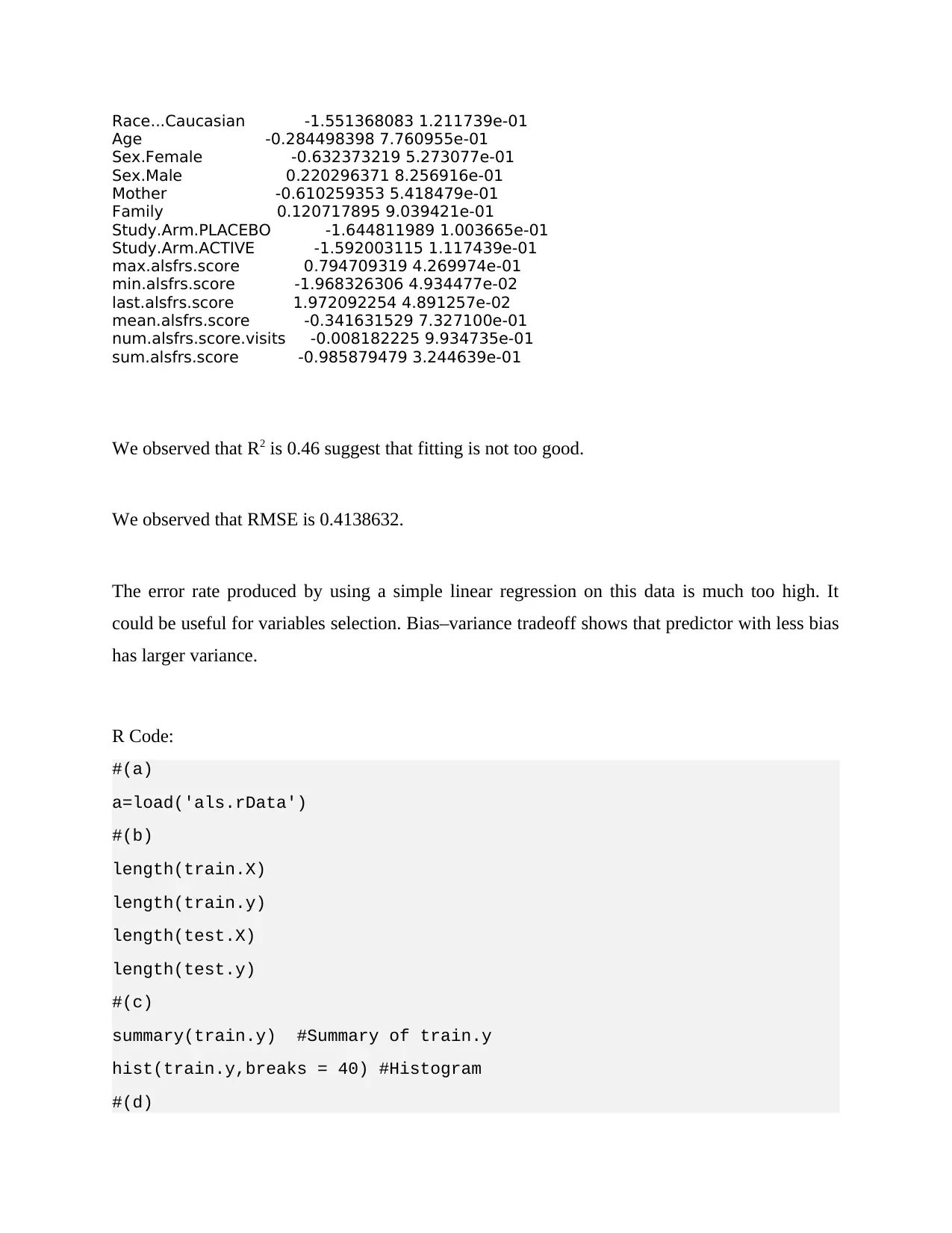
This document provides a comprehensive solution to Problem Set 1 for the STATS216v Introduction to Statistical Learning course at Stanford University, Summer 2018. The solution addresses various aspects of statistical learning, including supervised and unsupervised learning models. It covers regression and classification problems, determining the number of observations and predictors in different scenarios. The assignment includes detailed explanations and analysis of different scenarios, such as oil excavation, advertisement targeting, and unemployment rate prediction. The solution also explores the use of flexible and inflexible regression models, discussing their performance based on the number of predictors and observations. Furthermore, it provides R code and output to analyze college data, including summary statistics, scatter plots, and histograms. The document also includes an analysis of a linear regression model applied to ALS data, covering coefficient estimates, R-squared, RMSE, and bias-variance trade-offs. The solution provides insights into the practical application of statistical learning concepts and techniques.

STATS216v Introduction to Statistical Learning
Stanford University, Summer 2018
Problem Set 1
Question 1:
1: (a)
This is supervised learning model. It is example of regression. We are interested in prediction.
We predict the most promising spot to dig. Here number of observations n = 80 and number of
predictors p = 24.
1: (b)
This is supervised learning model. It is example of classification. Here we are interested in
prediction. We predict the whether to display advertisement A or advertisement B to each
customer. Here number of observations n = 300 and number of predictors p = 3 (age, zip code,
and gender).
1: (c)
This is supervised learning model. It is example of regression. Here we are interested in
inference. We are interested in discovering factors that are associated with the unemployment
rate across different U.S. cities. Here number of observations n = 400 and number of predictors p
= 6 (the population, state, average income, crime rate, percentage of students who graduate high
school and unemployment level.).
1: (d)
This is unsupervised learning model. For the each students we don’t have responses (different
subtypes) of students in the application pool.

1 (e):
This is supervised learning model. It is example of classification. Here we are interested in
prediction. We predict the type of cells based on a few measurements. Here number of
observations n = 68 and number of predictors p = 3 (the number of branch points, the number of
active processes, and the average process length).
Question 2:
2 (a):
We preferred inflexible regression model as number of predictors (number of genes) p is
extremely large, and the number of observations (number of patients) n is small.
2 (b):
We preferred flexible regression model as number of predictors (math, science and history
grades in the 7th grade) p is small, and the number of observations (number of students) n is
extremely large.
2 (c):
We preferred inflexible regression model as we variation in data is more.
2 (d):
We preferred flexible regression model as we variation in data is less. Flexible model will
perform better to find non-linear effect also.

Question 3:
3 (a):
Flexible model performs better. A flexible models fits the data well with larger sample size and
performs better than inflexible model.
3 (b):
Flexible model performs worse. A flexible models overfit small number of observation.
3 (c):
Flexible model performs worse. A flexible method would fit to the noise in the error terms and
increase variance.
3 (d):
Flexible model performs better. A flexible models gets more degrees of freedom fits the data
well.
3 (e):
Flexible model performs worse as it would fit to the noise in the error terms and increase
variance.

Question 4:
Solution is obtained from R studio. Here we have given the some output of the program.
> summary(College)
Private Apps Accept Enroll Top10perc
No :212 Min. : 81 Min. : 72 Min. : 35 Min. : 1.00
Yes:565 1st Qu.: 776 1st Qu.: 604 1st Qu.: 242 1st Qu.:15.00
Median : 1558 Median : 1110 Median : 434 Median :23.00
Mean : 3002 Mean : 2019 Mean : 780 Mean :27.56
3rd Qu.: 3624 3rd Qu.: 2424 3rd Qu.: 902 3rd Qu.:35.00
Max. :48094 Max. :26330 Max. :6392 Max. :96.00
Top25perc F.Undergrad P.Undergrad Outstate Room.Board
Min. : 9.0 Min. : 139 Min. : 1.0 Min. : 2340 Min. :1780
1st Qu.: 41.0 1st Qu.: 992 1st Qu.: 95.0 1st Qu.: 7320 1st Qu.:3597
Median : 54.0 Median : 1707 Median : 353.0 Median : 9990 Median :4200
Mean : 55.8 Mean : 3700 Mean : 855.3 Mean :10441 Mean :4358
3rd Qu.: 69.0 3rd Qu.: 4005 3rd Qu.: 967.0 3rd Qu.:12925 3rd Qu.:5050
Max. :100.0 Max. :31643 Max. :21836.0 Max. :21700 Max. :8124
Books Personal PhD Terminal S.F.Ratio
Min. : 96.0 Min. : 250 Min. : 8.00 Min. : 24.0 Min. : 2.50
1st Qu.: 470.0 1st Qu.: 850 1st Qu.: 62.00 1st Qu.: 71.0 1st Qu.:11.50
Median : 500.0 Median :1200 Median : 75.00 Median : 82.0 Median :13.60
Mean : 549.4 Mean :1341 Mean : 72.66 Mean : 79.7 Mean :14.09
3rd Qu.: 600.0 3rd Qu.:1700 3rd Qu.: 85.00 3rd Qu.: 92.0 3rd Qu.:16.50
Max. :2340.0 Max. :6800 Max. :103.00 Max. :100.0 Max. :39.80
perc.alumni Expend Grad.Rate
Min. : 0.00 Min. : 3186 Min. : 10.00
1st Qu.:13.00 1st Qu.: 6751 1st Qu.: 53.00
Median :21.00 Median : 8377 Median : 65.00
Mean :22.74 Mean : 9660 Mean : 65.46
3rd Qu.:31.00 3rd Qu.:10830 3rd Qu.: 78.00
Max. :64.00 Max. :56233 Max. :118.00
>

> length(which(College$Private=="Yes"))
[1] 565
Out of 777, 565 colleges are private whereas 212 are non-private.
> length(which(College$Elite=="Yes"))
[1] 78
There are 78 elite universities.

R Code:
# Set the working directory
# Read the data
College=read.csv('College.csv',header=1)
#To view the data
View(College)
#For removing first column
rownames(College)= College[,1]
College=College[,-1]
View(College )
#Summary of Data
summary(College)
#scatterplot of the column PhD versus the column Grad.Rate.
plot(College$Grad.Rate,College$PhD,xlab="Grad.Rate",ylab="PhD",main="Scatter
Plot")
#Number of Private Colleges
length(which(College$Private=="Yes"))
#(g)
Elite=rep("No",nrow (College))
Elite[College$Top10perc>50]="Yes"
Elite=as.factor(Elite)

College=data.frame(College,Elite)
#How many elite universities are there?
length(which(College$Elite=="Yes"))
#Box Plot
plot(College$Elite, College$Outstate, xlab = "Elite University", ylab ="Out of
State tuition in USD", main = "Outstate Tuition Plot")
# (h) Histogram
par(mfrow=c(2,2))
hist(College$Top10perc, col = 4, xlab = "Top 10%", ylab = "Count",main="")
hist(College$Top25perc, col = 6, xlab = "Top 25%", ylab = "Count",main="")
hist(College$Books, col = 2, xlab = "Books", ylab = "Count",main="")
hist(College$PhD, col = 3, xlab = "PhD", ylab = "Count",main="")
Question 5:
One can see that variable is negatively skewed.

One can study the relation between different predictors by observing the above scatter plots of
predictors.
(e)
> coef(summary(lm.model))[1:20,1:4]
Estimate Std. Error
(Intercept) 5.2523261623 1.005248e+01
Onset.Delta -0.0004375411 4.516149e-05
Symptom.Speech -0.0225458435 9.120369e-02
Symptom.WEAKNESS -0.1030724618 8.140383e-02
Site.of.Onset.Onset..Bulbar -0.3672390249 2.492628e-01
Site.of.Onset.Onset..Limb -0.2722652619 2.516364e-01
Race...Caucasian -0.1472308983 9.490391e-02
Age -0.0005163468 1.814937e-03
Sex.Female -0.0605416162 9.573716e-02
Sex.Male 0.0195376288 8.868793e-02
Mother -0.0462694066 7.581925e-02
Family 0.0067961369 5.629768e-02
Study.Arm.PLACEBO -3.1549354316 1.918113e+00
Study.Arm.ACTIVE -3.0519454033 1.917047e+00
max.alsfrs.score 0.0622267218 7.830124e-02
min.alsfrs.score -0.1666353650 8.465840e-02
last.alsfrs.score 0.4090457993 2.074172e-01
mean.alsfrs.score -0.1208903623 3.538618e-01
num.alsfrs.score.visits -0.0058420080 7.139877e-01
sum.alsfrs.score -0.0778763045 7.899171e-02
t value Pr(>|t|)
(Intercept) 0.522490777 6.014605e-01
Onset.Delta -9.688368476 3.700894e-21
Symptom.Speech -0.247203188 8.048088e-01
Symptom.WEAKNESS -1.266186858 2.057820e-01
Site.of.Onset.Onset..Bulbar -1.473300789 1.410284e-01
Site.of.Onset.Onset..Limb -1.081979013 2.795589e-01

Race...Caucasian -1.551368083 1.211739e-01
Age -0.284498398 7.760955e-01
Sex.Female -0.632373219 5.273077e-01
Sex.Male 0.220296371 8.256916e-01
Mother -0.610259353 5.418479e-01
Family 0.120717895 9.039421e-01
Study.Arm.PLACEBO -1.644811989 1.003665e-01
Study.Arm.ACTIVE -1.592003115 1.117439e-01
max.alsfrs.score 0.794709319 4.269974e-01
min.alsfrs.score -1.968326306 4.934477e-02
last.alsfrs.score 1.972092254 4.891257e-02
mean.alsfrs.score -0.341631529 7.327100e-01
num.alsfrs.score.visits -0.008182225 9.934735e-01
sum.alsfrs.score -0.985879479 3.244639e-01
We observed that R2 is 0.46 suggest that fitting is not too good.
We observed that RMSE is 0.4138632.
The error rate produced by using a simple linear regression on this data is much too high. It
could be useful for variables selection. Bias–variance tradeoff shows that predictor with less bias
has larger variance.
R Code:
#(a)
a=load('als.rData')
#(b)
length(train.X)
length(train.y)
length(test.X)
length(test.y)
#(c)
summary(train.y) #Summary of train.y
hist(train.y,breaks = 40) #Histogram
#(d)

colnames(train.X)[1:20]
pairs(train.X[,21:25])
#Fitting of Regression model
lm.model=lm(train.y ~., data = data.frame(train.y,train.X))
#First 20 coefficients
coef(summary(lm.model))[1:20,1:4]
#R squared
summary(lm.model)$r.squared
pred=predict(lm.model)
#RMSE
RMSE=sqrt(mean((pred-train.y)^2))
RMSE
Reference:
James, G., Witten, D., Hastie, T. and Tibshirani, R., 2013. An introduction to statistical learning
(Vol. 112). New York: springer.
Montgomery, D.C., Peck, E.A. and Vining, G.G., 2012. Introduction to linear regression
analysis (Vol. 821). John Wiley & Sons.