Financial Modeling: Stochastic Volatility and Option Pricing
VerifiedAdded on 2023/04/20
|15
|3405
|413
Homework Assignment
AI Summary
This assignment solution delves into the application of stochastic volatility models in option pricing, specifically focusing on the Stein model and its characteristics. It involves forming a risk-free portfolio considering the stochastic dynamics of variance. The solution applies numerical parameters to analyze the volatility risk, utilizing concepts such as Fourier transforms and characteristic functions to derive option pricing methodologies. It explores the probability measure using the Radon-Nikodym derivative and includes calculations for call price models under different conditions and parameter values. The assignment also presents graphical analyses to represent the impact of varying parameters on option prices. Desklib offers this solved assignment and other study resources for students.

Admin
[COMPANY NAME] [Company address]
[COMPANY NAME] [Company address]
Paraphrase This Document
Need a fresh take? Get an instant paraphrase of this document with our AI Paraphraser

Contents
Question 1.............................................................................................................................................1
Question 2.............................................................................................................................................5
Question 3.............................................................................................................................................7
Question 4.............................................................................................................................................8
Question 5.............................................................................................................................................9
Question 6...........................................................................................................................................11
Question 1
Let St
(0):=1 denote the underlying asset process and Stein model of the variance process. The
general form of stochastic volatility model is characterized by σ t is being the expected rate of
return process, where Xt is denoting the dividend yield βSS being the volatility of variance.
KSS is the speed of mean reversion BQ and W Qare two independent Q-Brownian motions
generating the filtration Ft, dθSS, which is the mean reversion level. Ft , t∈[0,T] with T>0
possibly has correlated with EQ[(ST −k )+¿∨Ft ¿]. The general form of a stochastic volatility
model is,
dSt:=σ t St dBt
Q, S0>0,
dσ t:= KSS(θSS−σ t)dt+ βSS( ρSS dBt
Q+√ 1−ρSS
2 dW t
Q), σ 0>0,
The equation is obtained by forming a risk-free portfolio, where this time it involves a
position in an extra derivative as compared to the constant volatility case, due to the second
source of randomness, or namely the variance stochastic dynamics. The price of a derivative
contract V should be satisfied.
dσ t:= KSS (θSS−σ t)dt+βSS(ρSS dBt
Q+√1−ρSS
2 dW t
Q), σ 0>0
Let us apply the values of numerical parameters as follows,
S0:= 100, σ 0:=θSS ≔0.1, KSS ≔2 , ρSS:=0.5 βSS:=0.05, T:=1 ρS:=0.5
dσ t: = 2 (0.1−σt ) dt+0.05 (0.5 dBt
Q+√1−(0.5)2 dW t
Q), σ 0>0
∂ σ
∂ t =2 ( 0.1−σt ) ∂ σ
∂ t +0.05 (0.5 ∂ B
∂ t +
√ 1−(0.5)2 ∂W
∂t ), σ 0>0
∂ σ
∂ t =2 ( 0.1−σt ) ∂ σ
∂ t +0.05 (0.5 ∂ B
∂ t + 1
2(1-(0.5)2) ∂W
∂t
Where, βSS( ρSS dBt
Q+√ 1−ρSS
2 dW t
Q), is the market price of volatility risk and r is the risk free
rate. For bearing the additional volatility risk, investors require extra return of amount ψSS(u;t,
σ t , xt )
The general definition will be presented. The option pricing methodology, which will be
discussed in the Fourier transform of a real function is ψSS(u;t,σ , x,x.
ψSS(u;t,σ t , xt ): = EQ[eiu X T
∨Ft]
⊘ This is a preview!⊘
Do you want full access?
Subscribe today to unlock all pages.
Trusted by 1+ million students worldwide

With i being the imaginary unit, and u being a real number (u ∈ R). In case F( xt)=f XT ( x ) is a
probability density function of a random variable X, the transform above is the characteristic
function of X to be denoted by ϕX(u).
Random variables are fully described by their characteristic functions, that is, if ϕX(u) is
known then the distribution of X is completely defined. Also, by knowing the characteristic
function,
CSS(t, S, σ):= EQ[(ST −k )+¿∨Ft ¿], t∈[0,T]
C= EQ[eiu X T
∨Ft]
f XT ( x )=F−1[ϕX(u)]du= 1
√ 2 π ∫
0
T
eiu X T
σ X(u)du
CT(k)= EQ[eiu X T
∨Ft]
Thus, we can consider the call Price's model of the ODE for C, D and E such as for all
u∈R and all t∈ [0, T] the equation is,
ψSS(u;t,σ t , xt )= exp(c(u, T-t)+ D(u, T-t) σ + 1
2 E ( u ,T −t ) σ2 +iux)
Let us consider the value of C (u,0) where u∈R
C (u,T-t)=EQ[(ST −k )+¿¿| 1
2 σ ∫
0
T
eiu X T
σ X(u)du
X=log ST k=log k σ (X)are the risk natural values of the call price,
C (u,T-t)=EQ[(ST −k )+¿¿| 1
2 σ ∫
0
T
ex−ek q(x)dx
lim
k → ∞
CT (k )=s0
Let us consider the limit values as, T>0
ψSS = σt (S−(T +1) xt)
T 2+T −s2+ i(2T +1) s
Paraphrase This Document
Need a fresh take? Get an instant paraphrase of this document with our AI Paraphraser

=∫
0
T
eisk ψ ( s)ds
Let us consider the local variable,
^w(T-k)=∫
0
T
ei (T −t)k ψ (T −k )ds
^w(T-k)=∫
0
T
ei ( T −t ) k (eT −K )+¿dt
C(u,T-t)= K i ( T−k ) +1
(T −t)2 −i( T −t)
Let us consider the value of D (u,0) where u∈R
D (u,T-t)=EQ[(ST −k )+¿¿| 1
2 σ ∫
0
T
eiu X T
σ X(u)du
X=log ST k=log k σ (X) are the risk natural values of the call price,
D (u,T-t)=EQ[(ST −k )+¿¿| 1
2 σ ∫
0
T
ex−ek q(x)dx
lim
k → ∞
CT (k )=s0
Let us consider the limit values as, T>0
ψSS = σt (S−(T +1) xt)
T 2+T −s2+ i(2T +1) s
=∫
0
T
eisk ψ ( s)ds
Let us consider the local variable,
^w(T-k)=∫
0
T
ei (T −t)k ψ (T −k )ds
0
T
eisk ψ ( s)ds
Let us consider the local variable,
^w(T-k)=∫
0
T
ei (T −t)k ψ (T −k )ds
^w(T-k)=∫
0
T
ei ( T −t ) k (eT −K )+¿dt
C(u,T-t)= K i ( T−k ) +1
(T −t)2 −i( T −t)
Let us consider the value of D (u,0) where u∈R
D (u,T-t)=EQ[(ST −k )+¿¿| 1
2 σ ∫
0
T
eiu X T
σ X(u)du
X=log ST k=log k σ (X) are the risk natural values of the call price,
D (u,T-t)=EQ[(ST −k )+¿¿| 1
2 σ ∫
0
T
ex−ek q(x)dx
lim
k → ∞
CT (k )=s0
Let us consider the limit values as, T>0
ψSS = σt (S−(T +1) xt)
T 2+T −s2+ i(2T +1) s
=∫
0
T
eisk ψ ( s)ds
Let us consider the local variable,
^w(T-k)=∫
0
T
ei (T −t)k ψ (T −k )ds

^w(T-k)=∫
0
T
ei ( T −t ) k (eT −K )+¿dt
D (u,T-t)= K i ( T−k ) +1
(T −t)2 −i( T −t)
Let us consider the value of E (u,0) where u∈R
1
2 E ( u ,T −t ) σ2 +iux= E (u,T-t) σ 2=EQ[(ST −k )+¿¿| 1
2∫
0
T
eiu X T
+iux σ 2X(u)du
X=log ST k=log k σ (X) is there risk natural values of the call price,
E (u,T-t)=EQ[(ST −k )+¿¿| 1
2∫
0
T
ex−ek +iux q(x)dx
lim
k → ∞
ET (k )=s0
Let as consider the limit values is, T>0
ψSS = σt (S−(T +1) xt)
T 2+ T −s2+ i(2T +1) s + 1
2 iux
=∫
0
T
eisk + 1
2 iux ψ (s)ds
Let us consider the local variable,
^w(T-k)=∫
0
T
ei (T −t)k + 1
2 iux ψ (T −k )ds
^w(T-k)=∫
0
T
ei ( T −t ) k ( eT −K ) + 1
2 iux
E (u ,T-t) = K i (T−k )+1
(T −t)2 −i(T −t)+ 1
2 iux
= K i (T−k )+1
(T −t )2 −i(T −t) + Ki (T −k )+ 1
( T −t)2−i(T −t) + Ki ( T−k )+1
(T −t)2−i(T −t )+ 1
2 iux
0
T
ei ( T −t ) k (eT −K )+¿dt
D (u,T-t)= K i ( T−k ) +1
(T −t)2 −i( T −t)
Let us consider the value of E (u,0) where u∈R
1
2 E ( u ,T −t ) σ2 +iux= E (u,T-t) σ 2=EQ[(ST −k )+¿¿| 1
2∫
0
T
eiu X T
+iux σ 2X(u)du
X=log ST k=log k σ (X) is there risk natural values of the call price,
E (u,T-t)=EQ[(ST −k )+¿¿| 1
2∫
0
T
ex−ek +iux q(x)dx
lim
k → ∞
ET (k )=s0
Let as consider the limit values is, T>0
ψSS = σt (S−(T +1) xt)
T 2+ T −s2+ i(2T +1) s + 1
2 iux
=∫
0
T
eisk + 1
2 iux ψ (s)ds
Let us consider the local variable,
^w(T-k)=∫
0
T
ei (T −t)k + 1
2 iux ψ (T −k )ds
^w(T-k)=∫
0
T
ei ( T −t ) k ( eT −K ) + 1
2 iux
E (u ,T-t) = K i (T−k )+1
(T −t)2 −i(T −t)+ 1
2 iux
= K i (T−k )+1
(T −t )2 −i(T −t) + Ki (T −k )+ 1
( T −t)2−i(T −t) + Ki ( T−k )+1
(T −t)2−i(T −t )+ 1
2 iux
⊘ This is a preview!⊘
Do you want full access?
Subscribe today to unlock all pages.
Trusted by 1+ million students worldwide
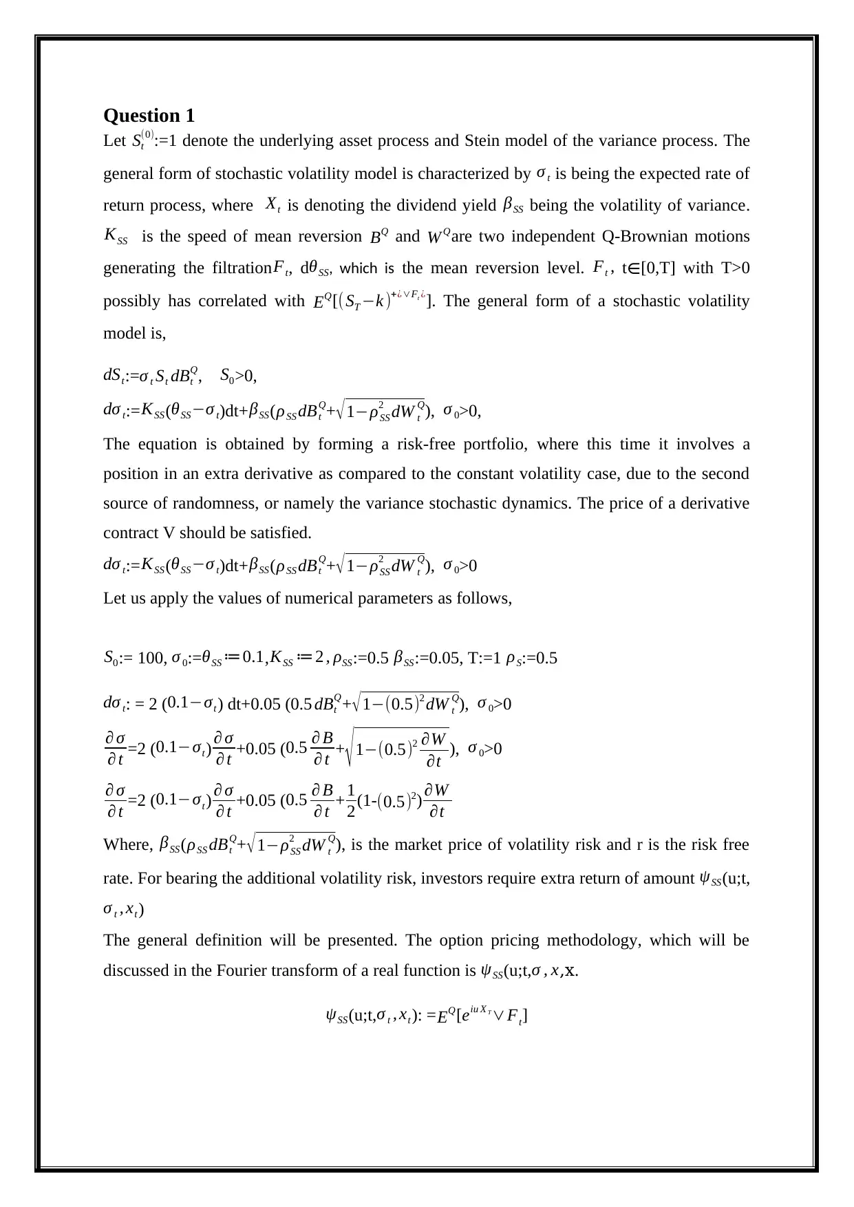
Xt :=log ( St
S0
) being the characteristic function of the standardized log-price at maturityXT - X 0
= log ( St
S0
), well as other important results regarding the practical implementation of the
Fourier transform apparatus can be found.
Question 2
a) f XT ( y ) y∈[-0.5,0.5] for ρSS ∈[−0.5,0,0 .5]
f XT ( y ) = 1
2 π ∫
❑
❑
e−iuy ψSS ( u ; 0 , σ0 , x0 )du ,y∈ R
f XT ( y )=F−1[ϕX(u)]du= 1
√ 2 π ∫
0
T
eiuy σ X(u)du
We can consider the equation as,
dσ t:= KSS (θSS−σ t)dt+βSS(ρSS dBt
Q+√1−ρSS
2 dW t
Q), σ 0>0,
f XT ( y ) y ∈ [-0.5,0.5] for ρSS ∈[−0.5,0,0 .5]
f XT ( y ) = 1
2 π ∫
❑
❑
e−(0.5)+√ 1−(−0.5)2 =1.818
f XT ( y ) = 1
2 π ∫
❑
❑
e−(0.5)+√1−(0)2 =3.589
S0
) being the characteristic function of the standardized log-price at maturityXT - X 0
= log ( St
S0
), well as other important results regarding the practical implementation of the
Fourier transform apparatus can be found.
Question 2
a) f XT ( y ) y∈[-0.5,0.5] for ρSS ∈[−0.5,0,0 .5]
f XT ( y ) = 1
2 π ∫
❑
❑
e−iuy ψSS ( u ; 0 , σ0 , x0 )du ,y∈ R
f XT ( y )=F−1[ϕX(u)]du= 1
√ 2 π ∫
0
T
eiuy σ X(u)du
We can consider the equation as,
dσ t:= KSS (θSS−σ t)dt+βSS(ρSS dBt
Q+√1−ρSS
2 dW t
Q), σ 0>0,
f XT ( y ) y ∈ [-0.5,0.5] for ρSS ∈[−0.5,0,0 .5]
f XT ( y ) = 1
2 π ∫
❑
❑
e−(0.5)+√ 1−(−0.5)2 =1.818
f XT ( y ) = 1
2 π ∫
❑
❑
e−(0.5)+√1−(0)2 =3.589
Paraphrase This Document
Need a fresh take? Get an instant paraphrase of this document with our AI Paraphraser
f XT ( y ) = 1
2 π ∫
❑
❑
e−(0.5)+√ 1−(0.5)2 =1.818
f XT ( y ) = 1
2 π ∫
❑
❑
e0.5+√ 1−(−0.5)2 =3.455
f XT ( y ) = 1
2 π ∫
❑
❑
e0.5+√1−(0)2 =3.5898
f XT ( y ) = 1
2 π ∫
❑
❑
e0.5+√ 1−(0.5)2 =3.455
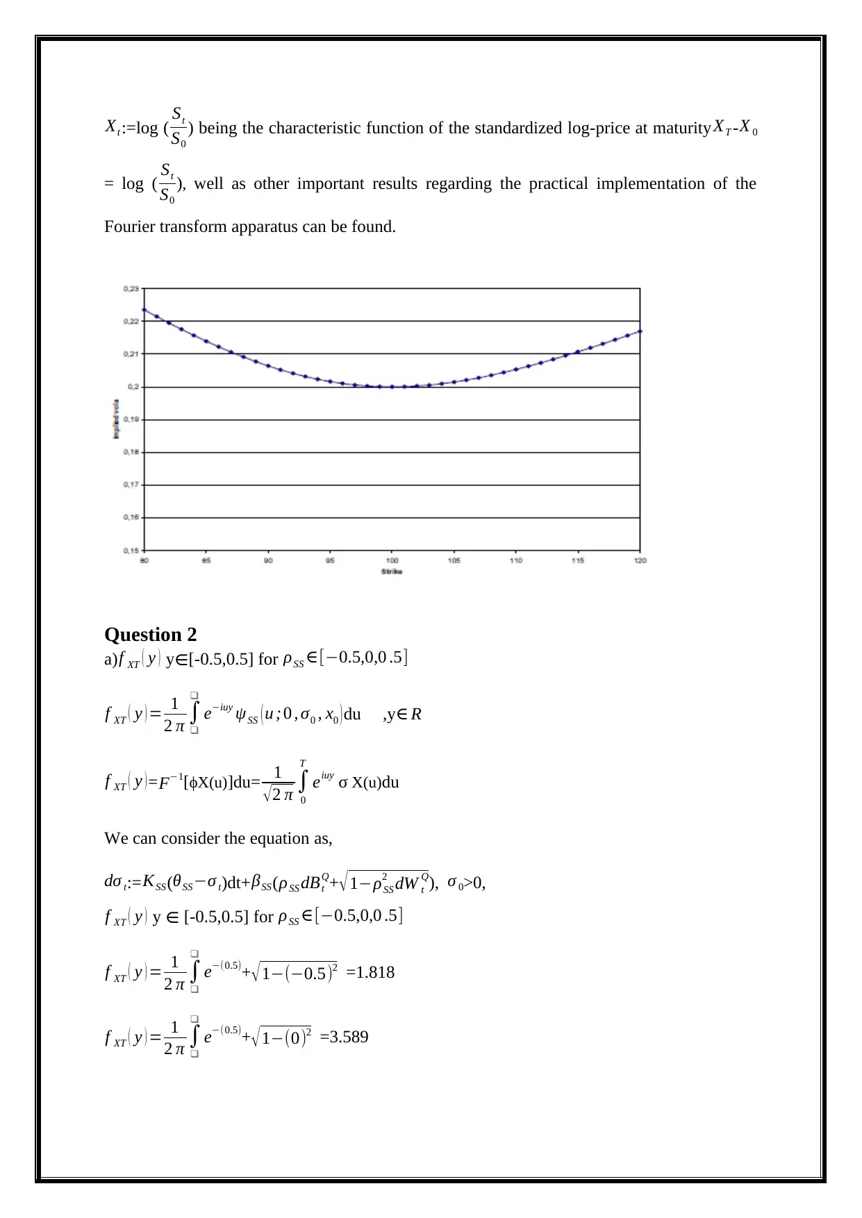
ρSS −0.5 0 0.5
-0.5 1.818 3.589 1.818
0.5 3.455 3.5898 3.455
0 2 4 6 8 10 12
0
2
4
6
8
10
12
𝑓_ ( )𝑋𝑇 𝑦
𝜌_𝑆𝑆
Y axis
b)
f XT ( y ) y ∈[-0.5,0.5] for ρSS ∈[0.01,0.05,0 .09]
f XT ( y ) = 1
2 π ∫
❑
❑
e−(0.5)+√ 1−(0.01)2 =1.952
Y
2 π ∫
❑
❑
e−(0.5)+√ 1−(0.5)2 =1.818
f XT ( y ) = 1
2 π ∫
❑
❑
e0.5+√ 1−(−0.5)2 =3.455
f XT ( y ) = 1
2 π ∫
❑
❑
e0.5+√1−(0)2 =3.5898
f XT ( y ) = 1
2 π ∫
❑
❑
e0.5+√ 1−(0.5)2 =3.455
ρSS −0.5 0 0.5
-0.5 1.818 3.589 1.818
0.5 3.455 3.5898 3.455
0 2 4 6 8 10 12
0
2
4
6
8
10
12
𝑓_ ( )𝑋𝑇 𝑦
𝜌_𝑆𝑆
Y axis
b)
f XT ( y ) y ∈[-0.5,0.5] for ρSS ∈[0.01,0.05,0 .09]
f XT ( y ) = 1
2 π ∫
❑
❑
e−(0.5)+√ 1−(0.01)2 =1.952
Y

f XT ( y ) = 1
2 π ∫
❑
❑
e(0.5 )+√1−(0.01)2 =3.589
f XT ( y ) = 1
2 π ∫
❑
❑
e−(0.5)+√1−(0.05)2 =1.951
f XT ( y ) = 1
2 π ∫
❑
❑
e(0.5 )+√1−(0.05)2 =3.588
f XT ( y ) = 1
2 π ∫
❑
❑
e−(0.5)+√1−(0.09)2 =1.948
f XT ( y ) = 1
2 π ∫
❑
❑
e(0.5 )+√1−(0.09)2 =3.585
ρSS 0.01 0.05 0.09
-0.5 1.952 3.589 1.951
0.5 3.588 1.948 3.585
0 2 4 6 8 10 12
0
2
4
6
8
10
12
pss
Y axis
Question 3
Probability measure ~
Q by the Radon-Nikodym derivative.
We can find the values of the current price's value and measure the ~
Q probability by using
the Radon –Nikodym derivative.
Y
2 π ∫
❑
❑
e(0.5 )+√1−(0.01)2 =3.589
f XT ( y ) = 1
2 π ∫
❑
❑
e−(0.5)+√1−(0.05)2 =1.951
f XT ( y ) = 1
2 π ∫
❑
❑
e(0.5 )+√1−(0.05)2 =3.588
f XT ( y ) = 1
2 π ∫
❑
❑
e−(0.5)+√1−(0.09)2 =1.948
f XT ( y ) = 1
2 π ∫
❑
❑
e(0.5 )+√1−(0.09)2 =3.585
ρSS 0.01 0.05 0.09
-0.5 1.952 3.589 1.951
0.5 3.588 1.948 3.585
0 2 4 6 8 10 12
0
2
4
6
8
10
12
pss
Y axis
Question 3
Probability measure ~
Q by the Radon-Nikodym derivative.
We can find the values of the current price's value and measure the ~
Q probability by using
the Radon –Nikodym derivative.
Y
⊘ This is a preview!⊘
Do you want full access?
Subscribe today to unlock all pages.
Trusted by 1+ million students worldwide
d ~
Q=ST =σ t St dBt
Q
d Q= S0 =σt S0 dBt
Q=σ t dBt
Q
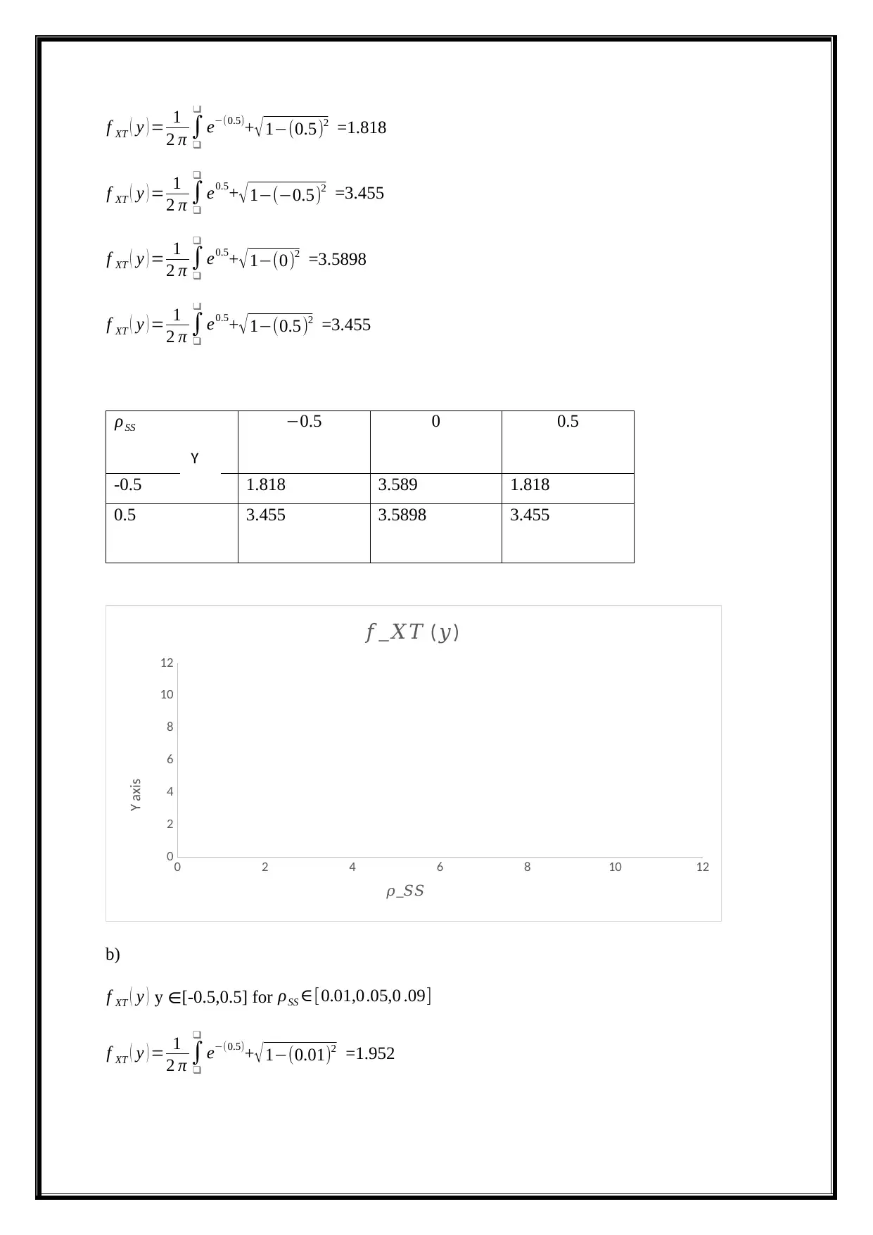
We can apply the dynamic values of Girsanov's theorem Let us consider the {dBt
Q} as the
wiener process on the probability space as {σ , F , ~
Q } and measure the process of the adapted
natural filtration of the values as S0 =¿{Ft
dB}
d ~
Q
d Q := ST
S0
=EQ ¿ ¿
0 2 4 6 8 10 12
0
2
4
6
8
10
12
probability measure of call price
Series1 Series2 Series3 Series4 Series5 Series6
dQ'=s0
dQ=st
Question 4
CSS(t, S, σ)= St
~
Q(ST ≥ k ∨Ft )-KQ ¿ ¿)
CSS(t, S, σ):=EQ[(ST ≥ k )+¿∨ Ft ¿] t∈[0,T]
~
C=EQ[eiu X T
∨Ft]- KQ ¿ ¿)
f XT ( x )= F−1[ϕX(u)]du= 1
√2 π ∫
0
T
eiu X T
σ X(u)du
Q=ST =σ t St dBt
Q
d Q= S0 =σt S0 dBt
Q=σ t dBt
Q
We can apply the dynamic values of Girsanov's theorem Let us consider the {dBt
Q} as the
wiener process on the probability space as {σ , F , ~
Q } and measure the process of the adapted
natural filtration of the values as S0 =¿{Ft
dB}
d ~
Q
d Q := ST
S0
=EQ ¿ ¿
0 2 4 6 8 10 12
0
2
4
6
8
10
12
probability measure of call price
Series1 Series2 Series3 Series4 Series5 Series6
dQ'=s0
dQ=st
Question 4
CSS(t, S, σ)= St
~
Q(ST ≥ k ∨Ft )-KQ ¿ ¿)
CSS(t, S, σ):=EQ[(ST ≥ k )+¿∨ Ft ¿] t∈[0,T]
~
C=EQ[eiu X T
∨Ft]- KQ ¿ ¿)
f XT ( x )= F−1[ϕX(u)]du= 1
√2 π ∫
0
T
eiu X T
σ X(u)du
Paraphrase This Document
Need a fresh take? Get an instant paraphrase of this document with our AI Paraphraser
CT(k)=EQ[eiu X T
∨Ft]- KQ ¿ ¿)
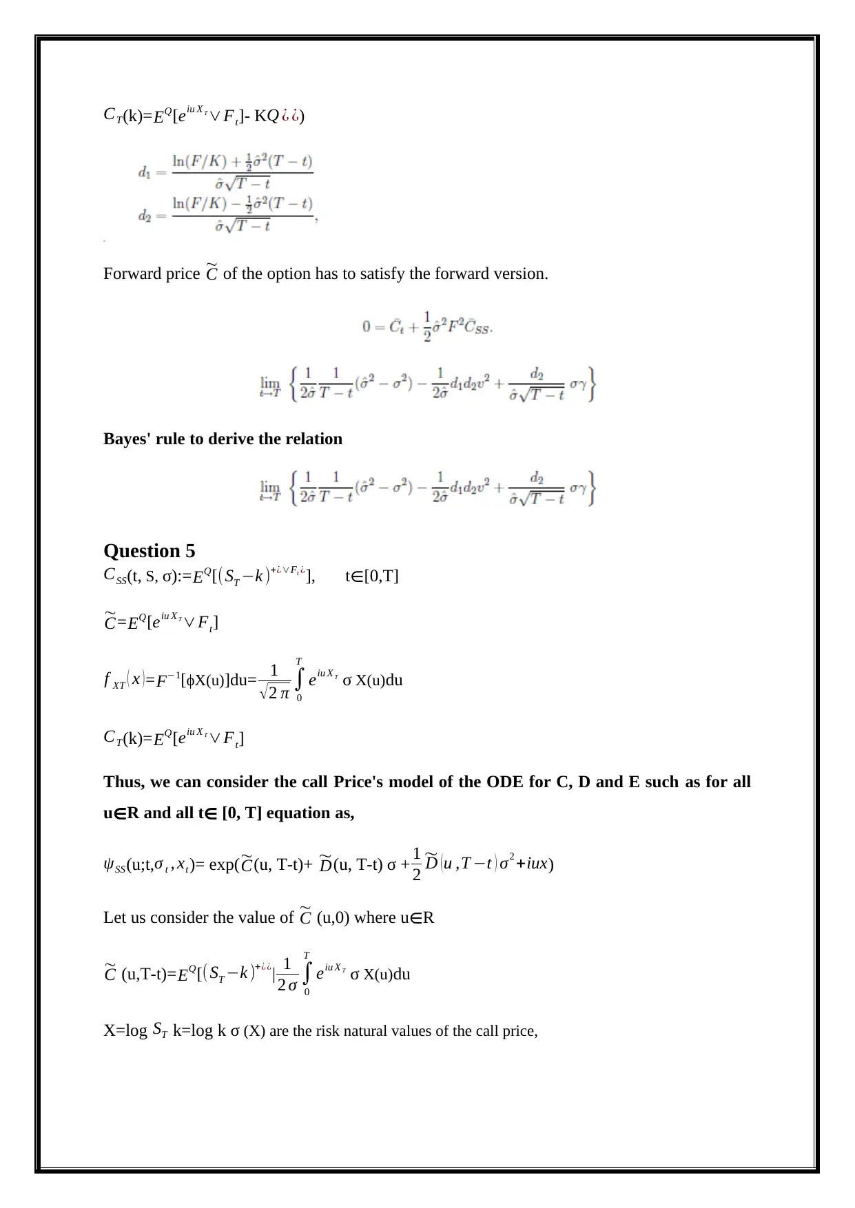
Forward price ~
C of the option has to satisfy the forward version.
Bayes' rule to derive the relation
Question 5
CSS(t, S, σ):=EQ[(ST −k )+¿∨Ft ¿], t∈[0,T]
~
C=EQ[eiu X T
∨Ft]
f XT ( x )= F−1[ϕX(u)]du= 1
√2 π ∫
0
T
eiu X T
σ X(u)du
CT(k)=EQ[eiu X T
∨Ft]
Thus, we can consider the call Price's model of the ODE for C, D and E such as for all
u∈R and all t∈ [0, T] equation as,
ψSS(u;t, σ t , xt )= exp( ~
C(u, T-t)+ ~
D(u, T-t) σ + 1
2
~
D (u ,T −t ) σ2 +iux)
Let us consider the value of ~
C (u,0) where u∈R
~
C (u,T-t)= EQ[(ST −k )+¿¿| 1
2 σ ∫
0
T
eiu X T
σ X(u)du
X=log ST k=log k σ (X) are the risk natural values of the call price,
∨Ft]- KQ ¿ ¿)
Forward price ~
C of the option has to satisfy the forward version.
Bayes' rule to derive the relation
Question 5
CSS(t, S, σ):=EQ[(ST −k )+¿∨Ft ¿], t∈[0,T]
~
C=EQ[eiu X T
∨Ft]
f XT ( x )= F−1[ϕX(u)]du= 1
√2 π ∫
0
T
eiu X T
σ X(u)du
CT(k)=EQ[eiu X T
∨Ft]
Thus, we can consider the call Price's model of the ODE for C, D and E such as for all
u∈R and all t∈ [0, T] equation as,
ψSS(u;t, σ t , xt )= exp( ~
C(u, T-t)+ ~
D(u, T-t) σ + 1
2
~
D (u ,T −t ) σ2 +iux)
Let us consider the value of ~
C (u,0) where u∈R
~
C (u,T-t)= EQ[(ST −k )+¿¿| 1
2 σ ∫
0
T
eiu X T
σ X(u)du
X=log ST k=log k σ (X) are the risk natural values of the call price,

~
C (u,T-t)=EQ[(ST −k )+¿¿| 1
2 σ ∫
0
T
ex−ek q(x)dx
lim
k → ∞
~
CT (k )=s0
Let us consider the limit values as, T>0
ψSS = σt (S−(T +1) xt)
T 2+T −s2+ i(2T +1) s
=∫
0
T
eisk ψ ( s)ds
Let us consider the local variable,
^w(T-k)=∫
0
T
ei (T −t)k ψ (T −k )ds
^w(T-k)=∫
0
T
ei ( T −t ) k (eT −K )+¿dt
~
C(u,T-t)= K i ( T−k ) +1
(T −t)2 −i( T −t)
Let us consider the value of D (u,0) where u∈R.
~
D (u,T-t)=EQ[( ST −k )+¿¿| 1
2 σ ∫
0
T
eiu X T
σ X(u)du
X=log ST k=log k σ (X) are the risk natural values of the call price,
~
D(u,T-t)=EQ[( ST −k )+¿¿| 1
2 σ ∫
0
T
ex−ek q(x)dx
lim
k → ∞
~
DT (k )= s0
Let us consider the limit values as, T>0
⊘ This is a preview!⊘
Do you want full access?
Subscribe today to unlock all pages.
Trusted by 1+ million students worldwide
1 out of 15
Your All-in-One AI-Powered Toolkit for Academic Success.
+13062052269
info@desklib.com
Available 24*7 on WhatsApp / Email
![[object Object]](/_next/static/media/star-bottom.7253800d.svg)
Unlock your academic potential
Copyright © 2020–2026 A2Z Services. All Rights Reserved. Developed and managed by ZUCOL.