Statistical Inference & Regression Analysis on Stock Analysis
VerifiedAdded on 2020/05/16
|9
|2780
|61
Report
AI Summary
This report presents a statistical analysis of IBM and Boeing stocks, comparing their performance using historical data and financial modeling techniques. The analysis begins with data exploration, examining closing prices and identifying trends. It then delves into return analysis, calculating mean, standard deviation, and other statistical measures to assess risk and potential returns. The report utilizes the Jarque-Bera test to assess the normality of returns, which informs the choice of statistical tests. Hypothesis testing is employed to evaluate claims about average returns and to compare the risk profiles of the two stocks, including the use of F-tests and z-tests. Furthermore, the report incorporates regression analysis to estimate beta, R-squared, and the relationship between stock returns and the S&P 500, culminating in a Capital Asset Pricing Model (CAPM) analysis. The conclusion summarizes the findings, highlighting the relative performance and risk characteristics of IBM and Boeing, and offering investment insights. The report uses Excel for data analysis and Yahoo Finance for data collection.
Statistical Inference & Regression Analysis Report
On
Stock Analysis
(IBM Vs Boeing
using S & P 500)
1
On
Stock Analysis
(IBM Vs Boeing
using S & P 500)
1
Paraphrase This Document
Need a fresh take? Get an instant paraphrase of this document with our AI Paraphraser
Abstract
This analysis is done to understand the various parameters before investing in any stocks. The
requirements for this analysis are done using Excel Data Analysis. The data is used from yahoo for
reading the historical data of stock closing prices of Boeing & IBM, the standard index used as
market portfolio and the interest rate on 10-year US treasury bill used as an interest-free rate. This
study has used the concepts and models of statistical inference and financial model.
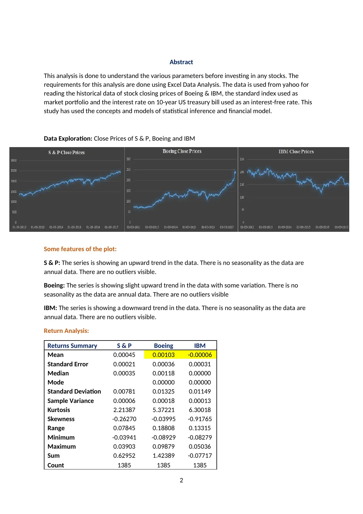
Data Exploration: Close Prices of S & P, Boeing and IBM
Some features of the plot:
S & P: The series is showing an upward trend in the data. There is no seasonality as the data are
annual data. There are no outliers visible.
Boeing: The series is showing slight upward trend in the data with some variation. There is no
seasonality as the data are annual data. There are no outliers visible
IBM: The series is showing a downward trend in the data. There is no seasonality as the data are
annual data. There are no outliers visible.
Return Analysis:
Returns Summary S & P Boeing IBM
Mean 0.00045 0.00103 -0.00006
Standard Error 0.00021 0.00036 0.00031
Median 0.00035 0.00118 0.00000
Mode 0.00000 0.00000
Standard Deviation 0.00781 0.01325 0.01149
Sample Variance 0.00006 0.00018 0.00013
Kurtosis 2.21387 5.37221 6.30018
Skewness -0.26270 -0.03995 -0.91765
Range 0.07845 0.18808 0.13315
Minimum -0.03941 -0.08929 -0.08279
Maximum 0.03903 0.09879 0.05036
Sum 0.62952 1.42389 -0.07717
Count 1385 1385 1385
2
This analysis is done to understand the various parameters before investing in any stocks. The
requirements for this analysis are done using Excel Data Analysis. The data is used from yahoo for
reading the historical data of stock closing prices of Boeing & IBM, the standard index used as
market portfolio and the interest rate on 10-year US treasury bill used as an interest-free rate. This
study has used the concepts and models of statistical inference and financial model.
Data Exploration: Close Prices of S & P, Boeing and IBM
Some features of the plot:
S & P: The series is showing an upward trend in the data. There is no seasonality as the data are
annual data. There are no outliers visible.
Boeing: The series is showing slight upward trend in the data with some variation. There is no
seasonality as the data are annual data. There are no outliers visible
IBM: The series is showing a downward trend in the data. There is no seasonality as the data are
annual data. There are no outliers visible.
Return Analysis:
Returns Summary S & P Boeing IBM
Mean 0.00045 0.00103 -0.00006
Standard Error 0.00021 0.00036 0.00031
Median 0.00035 0.00118 0.00000
Mode 0.00000 0.00000
Standard Deviation 0.00781 0.01325 0.01149
Sample Variance 0.00006 0.00018 0.00013
Kurtosis 2.21387 5.37221 6.30018
Skewness -0.26270 -0.03995 -0.91765
Range 0.07845 0.18808 0.13315
Minimum -0.03941 -0.08929 -0.08279
Maximum 0.03903 0.09879 0.05036
Sum 0.62952 1.42389 -0.07717
Count 1385 1385 1385
2
The data of 1385 observations are considered to analyse the adjusting returns. The average returns
of Boeing taken from this sample is 10% while the average returns of IBM are -0.01%. The variation
in the returns from the mean is about 13% in Boeing while its 11% in IBM. These statistics give an
indication that investing in Boeing will give better returns compared to investment done in IBM.
Higher returns are accompanied by higher risk. Investment is Boeing will be riskier compared to IBM
because the average return in Boeing is high when compared with IBM. Risk shows the volatility of
stocks compared to market and here, Boeing is more volatile when compared to IBM.
Jarque-Bera test to check Normality distribution of returns of Boeing and IBM:
This test is done to confirm normality in large dataset. The formula for the Jarque-Bera test statistic
is:
JB = n [(√b1)2 / 6 + (b2 – 3)2 / 24]
Where, n is the sample size
√b1 is the sample skewness coefficient
b2 is the kurtosis coefficient
Null Hypothesis: The data is normally distributed, skewness is zero and excess kurtosis is zero.
Alternate Hypothesis: The data does not show normal distribution.
A normal distributed data will have a skew value of 0 and a kurtosis of 3. This test can be
compared with chi-square distribution with 2 degrees of freedom. The null hypothesis of
normality is rejected if the calculated test statistic will exceed critical value from the chi-square
distribution.
Level α Critical Value
0.10 4.61
0.05 5.99
0.01 9.21
Result: The value of Jarque-Bera test of normality for Boeing and IBM is very high and is > 1 and this
means that the null hypothesis is rejected and returns of Boeing & IBM is not normally distributed.
We do normality test to understand which set of tests are applicable and which we should not use. If
the data follows normal distribution, we can apply parametric tests, which in other case will not be
valid. If the data can closely resemble a Normal distribution, then the data and hence the process
can be defined as being in control.
Understanding the average returns of Boeing:
To confirm that the average returns on Boeing is at least 3%, we need to conduct the hypothesis to
prove this claim.
Test Statistic used: Left-tail (single tail) statistic Hypothesis Test
The test is left-tail because the comparison here is with less than values of H1: mean < 3%
3
⊘ This is a preview!⊘
Do you want full access?
Subscribe today to unlock all pages.
Trusted by 1+ million students worldwide
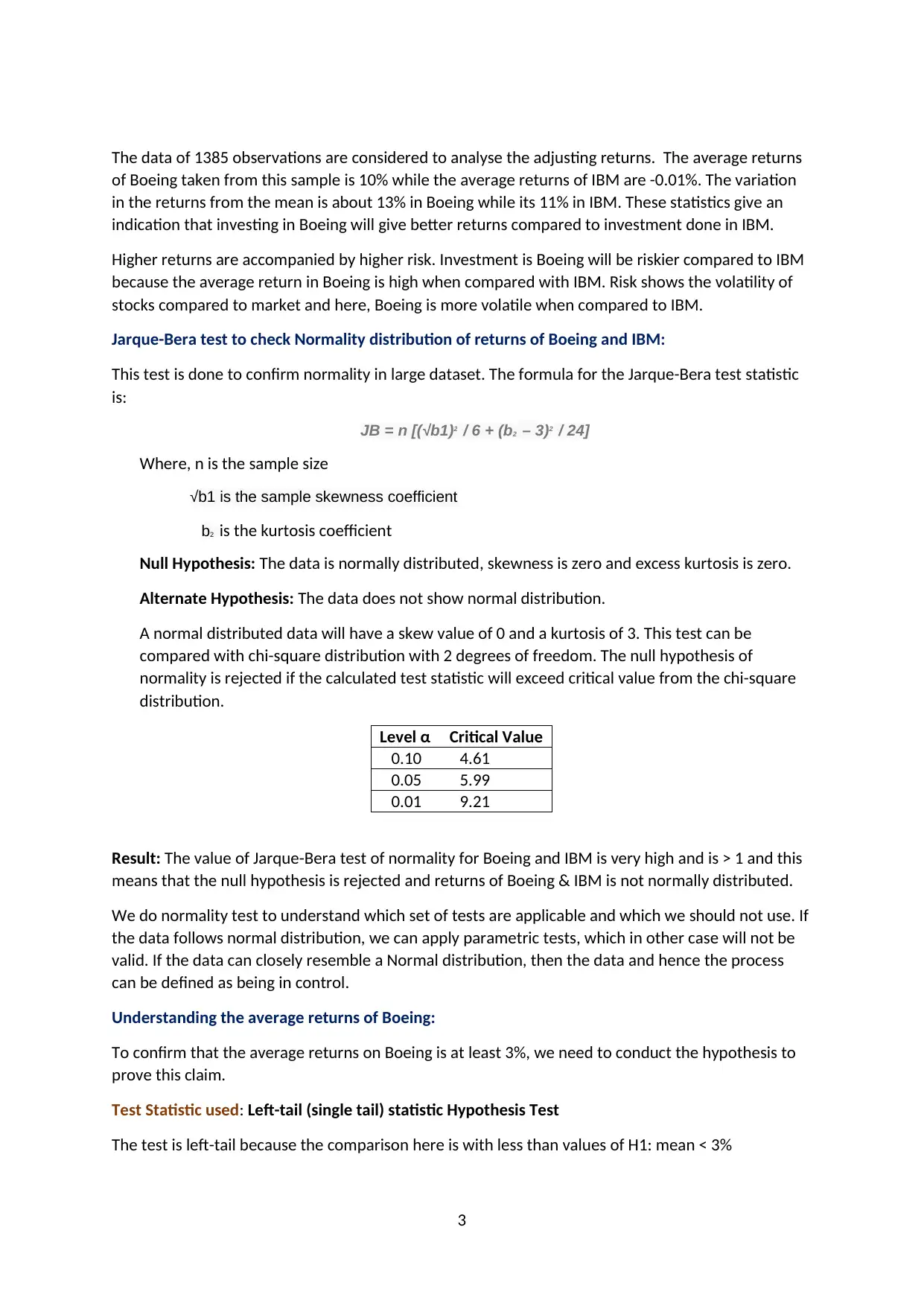
The taken level of significance is 5% and therefore the critical value becomes -1.645 as per z-value
for 45% area of the curve.
Rejection Region for Lower-Tailed Z Test (H1: μ < μ0 ) with α =0.05
The decision rule is: Reject H0 if Z < 1.645.
The calculated z-value is -81.40 which does not fall under the region and hence the null hypothesis is
not rejected. Based on our sample, we conclude that average return of Boeing is 3%.
Distribution of the test statistic under the null:
If the assumptions are true and H0 is accepted, the test statistic show normal distribution.
Risk:
Risk involves the chance in an individual’s actual return from the expected return. Before investing in
any stock, understanding of risk associated with returns on that stock is must.
Beta is a measure of risk in evaluation of stocks in comparison of market. Beta is calculated using
regression analysis and can also be calculated as per given formula.
According to market beta value is 1, and individual stocks are ranked according to how much they
deviate from the market. A stock which shift more than the market over time has a beta above 1.0
and the stock which moves less than the market, will have beta less than 1.0. High beta stocks are
riskier as they provide a potential for higher returns and low beta stocks have low risk and low
returns.
To analyse the associated risk, we conducted a hypothesis test using F-test to prove that variance in
returns of Boeing = variance in returns of IBM.
The level of significance considered is 5%. The critical value of F at 5% significance level is 2.20. If the
calculated test statistic value is more than the set critical value of 2.20, then we will reject null
hypothesis.
4
Paraphrase This Document
Need a fresh take? Get an instant paraphrase of this document with our AI Paraphraser
On calculation, we observed that the f-statistic value is 1.329 which does not fall in rejection region,
and hence we accept the null hypothesis.
We conclude by this that there is no significant variance in both the stocks i.e., Boeing & IBM.
Understanding mean population return of the stocks:
To understand the average population, return of the stocks, we had done a hypothesis test to study
the difference between the two population mean.
The test statistic used is two sample z test. The level of significance considered is 5%. The critical
values of z are -1.96 & +1.96. The calculated z statistic value if falls within this range of z values then
null hypothesis will be accepted else rejected.
This is 1 two-tail test and thus it has two rejection regions, one at each tail. The calculated z statistic
value is -0.6054 which does not fall under the rejection region and hence, we accept the null
hypothesis.
Based on our sample data of 67 observations, we conclude that average population return of Boeing
is equal to average population return of IBM.
Based on the hypothesis done above to ascertain the risk, average population mean & average
returns, it is evident that Boeing has better average returns compared to IBM, though there is not
much statistical evidence to show that investing in Boeing is better compared to investment in IBM.
Both the stocks have almost very close risk and very close average returns. According to my study,
investment in Boeing is better due to high Beta rate of 1 and high average returns when compared
with IBM.
Excess Returns:
The excess returns are the additional return that we get after subtracting the value of risk value
returns from the stock returns.
The excess market return is the additional return that is achieved after subtracting the value of risk
free returns from S & P 500 returns.
The risk-free return used here is 10-year treasury bill rate return.
CAPM using Regression Analysis:
The variables used in doing the regression analysis are:
Independent variable: The independent variable(s) is what you explain or predict the dependent
variable, and are usually represented by X. Here it is excess market return which is computed as
return on S & P minus the risk-free rate.
Dependent variable: The dependent variable is something you want to predict or explain, and is
usually represented by y. Here it is excess return on your preferred stock (Boeing).
Slope or coefficient: Amount of change in y when X changes by certain amount, denoted by Beta.
Constant: The constant term in the equation is the Y-intercept, denoted by Alpha.
The regression equation is:
5
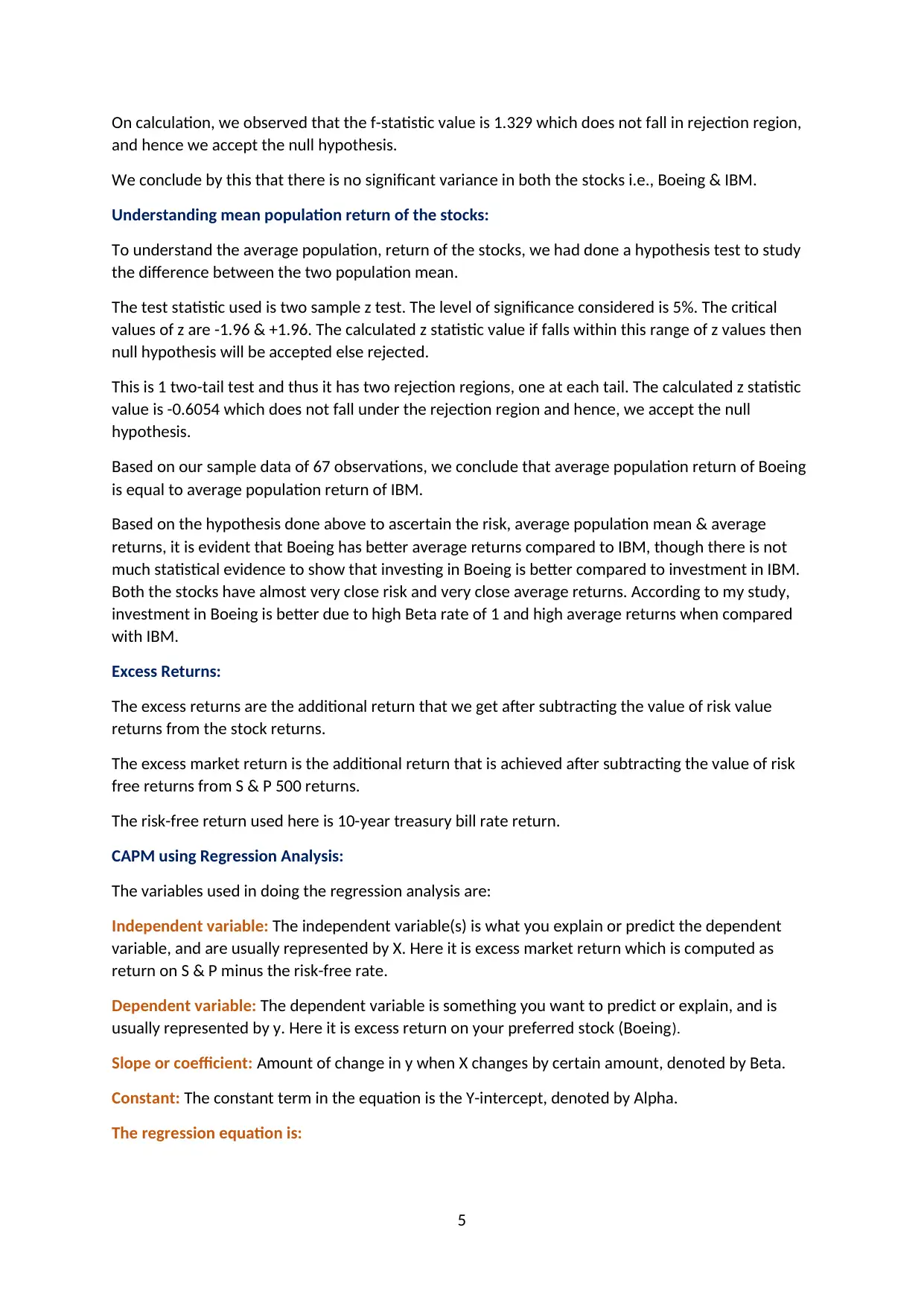
y = 1.0023x + 0.0006
R² = 0.9121
Scatter Plot: Relationship between S & P and Boeing returns
-0.20000 0.00000 0.20000 0.40000 0.60000 0.80000 1.00000 1.20000
-0.20000
0.00000
0.20000
0.40000
0.60000
0.80000
1.00000
1.20000
f(x) = 1.00233776483578 x + 0.000571336692890096
R² = 0.912144733942903
Regressing Boeing Excess Returns on the S & P 500,
2012-2017
S & P 500
Boeing
Slope Coefficient: 1.0023
With a unit increase in return on S & P (while keeping all other variables constant), the value of Boeing returns
increases by 1.0023 points. If the S & P returns 10, Boeing also returns 10 and vice-versa.
The relationship between the independent variable and the dependent variable is understood with the help of the
sign of the regression coefficient.
A regression coefficient of positive value indicates that with increase in the value of the independent
variable, the average value of the dependent variable will also increase.
A regression coefficient of negative value indicates that with decrease in the value of the independent
variable, the average value of the dependent variable will also decrease.
R-squared: 0.9121
The value of R-squared is always between 0% and 1%. The larger the value of R-squared the better the
regression line fits your observations. An R2 value near 1 is associated with a line that better fits the points. In
real-world, you will never see a regression line with an R-squared value of 1(100%).
Here, we’re trying to predict the relationship between S & P and Boeing risk free returns and the value of r-
squared tells that 91% of the variability in Boeing (out of 100%) is explained by the returns on S & P 500.
R-squared evaluates the scatter of the data points around the fitted regression line (y = 1.0023x + 0.0006).
R-squared value shows a relevant association between returns on S & P and the returns on Boeing as there is a
positive linear relationship between them as shown by the scatter plot.
Now, we will investigate the strength of this linear relationship by looking at the slope estimate. Since the slope
represents how much Y responds to change in X-value, lets calculate a 95% confidence interval for the slope,
and check whether it excludes 0. If it does, then we can rule out the chances that the slope is 0 and hence, we
can conclude that there is a significant linear relationship between them.
The slope estimate b tends to miss the true value(Beta) by an amount called the standard error of the slope and
the formula to calculate the confidence interval of the slope becomes:
95 Confidence interval calculation of slope:
6
⊘ This is a preview!⊘
Do you want full access?
Subscribe today to unlock all pages.
Trusted by 1+ million students worldwide
b1 ± t0.95, n-2SEb1
The calculated range of 95% confidence interval is: [0.99-1.015]
For each return on S & P, we can expect the return on Boeing in the range of [0.99-1.015]
We also observed that 0 is not contained in this interval as both units are positive, so we would reject the
idea that true slope is 0.
Thus, we conclude a significant relationship between returns on S & P & returns on Boeing.
Neutral Stock:
A stock with Beta equal to 1 is called neutral stock because it changes as the market change.
We have applied hypothesis testing using confidence interval to prove that the preferred stock-Boeing is
a neutral stock.
The test statistic used is a two-tail test. The confidence level considered is 95% and hence the level of
significance becomes 5%.
Confidence Intervals provide more information than calculated point estimates. Confidence intervals
for means are intervals constructed using a procedure that will contain the population mean a
specified proportion of time, typically either 95% or 99% of the time. These intervals are referred to
as 95% and 99% confidence intervals respectively.
There is a good reason to believe that the population mean return lies between these two bounds of
-0.04 (lower threshold) and 0.04(upper threshold) since 95% confidence intervals contain the true
mean.
If repeated samples were taken and the 95% confidence interval computed for each sample, 95% of
the intervals would contain the population mean return.
Ordinary Least Squares Method(OLS) in Regression Model:
A linear regression equation is written as:
Y =β0 + β1X + error(e)
The coefficient Beta(β) is found by minimizing the error of prediction (the difference between the real
value and the predicted value of Y) in this model.
We are interested to check the normality assumption of regression model here.
To estimate linear regression, we do not need data to be normal, but we assume that data is
normally distributed
If the assumption is true, then the observed residuals ei = Yi - Y^i should behave in a normal fashion
& the sum of residuals ei = 0
Method used is to plot the residuals against the values of X and check variance in plot.
We conclude that the applied method shows that the residuals when plotted against the value of X,
show variance which is constant and hence prove the normal distribution of error.
7
Paraphrase This Document
Need a fresh take? Get an instant paraphrase of this document with our AI Paraphraser
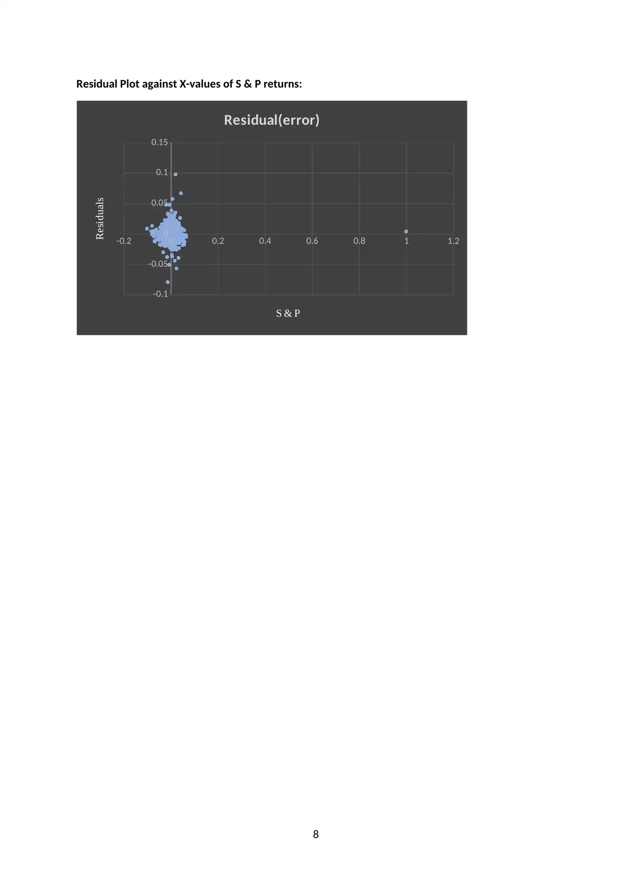
Residual Plot against X-values of S & P returns:
-0.2 0 0.2 0.4 0.6 0.8 1 1.2
-0.1
-0.05
0
0.05
0.1
0.15
Residual(error)
S & P
Residuals
8
-0.2 0 0.2 0.4 0.6 0.8 1 1.2
-0.1
-0.05
0
0.05
0.1
0.15
Residual(error)
S & P
Residuals
8
APPENDIX:
References:
Statistics Solutions (2013) What is Linear Regression? [online]
Available From: http://www.statisticssolutions.com/what-is-linear-regression/ [Accessed 21 January 2018]
Statistics How To (2018) Find a Linear Regression Equation[online]
Available From: http://www.statisticshowto.com/probability-and-statistics/regression-analysis/find-a-linear-
regression-equation/ [Accessed 21 January 2018]
Stat 501 Penn State Science[online]
Available From: https://onlinecourses.science.psu.edu/stat501/node/250 [Accessed 21 January 2018]
Lane, David M. Onlinestatbook [online]
Available From: http://onlinestatbook.com/2/regression/intro.html [Accessed 21 January 2018]
Minitab Express Support- Interpret the key results of Descriptive Statistics[online]
Available From:http://support.minitab.com/en-us/minitab-express/1/help-and-how-to/basic-statistics/summary-
statistics/descriptive-statistics/interpret-the-results/key-results/ [Accessed 21 January 2018]
Laerd statistics- Linear regression analysis using Stata [online]
Available From:https://statistics.laerd.com/stata-tutorials/linear-regression-using-stata.php
[Accessed 21 January 2018]
Stat 510 Penn State Science- Overview of Time Series Characteristics[online]
Available From: https://onlinecourses.science.psu.edu/stat510/node/47 [Accessed 6 February 2018]
Beta- Investopedia [online]
Available From: https://www.investopedia.com/terms/b/beta.asp [Accessed 7 February 2018]
Z-Test Investopedia [online]
Available From: https://www.investopedia.com/terms/z/z-test.asp [Accessed 6 February 2018]
Hypothesis Testing in Finance- Investopedia [online]
Available From: https://www.investopedia.com/articles/active-trading/092214/hypothesis-testing-
finance-concept-examples.asp [Accessed 5 February 2018]
Hypothesis Testing- Hypothesis Testing of a Single Population Mean- Kean University[online]
Available From: http://www.kean.edu/~fosborne/bstat/07amean.html [Accessed 6 February 2018]
Anandh, Saranya. Everything about Time Series Analysis (2016)- LinkedIn [Online]
Available From: https://www.linkedin.com/pulse/everything-time-series-analysis-components-data-
saranya-anandh/ [Accessed 4 February 2018]
Hypothesis Testing (2017)-Boston School of Public Health [online]
Available From: http://sphweb.bumc.bu.edu/otlt/MPH-Modules/BS/BS704_HypothesisTest-Means-
Proportions/BS704_HypothesisTest-Means-Proportions3.html [Accessed 5 February 2018]
9
⊘ This is a preview!⊘
Do you want full access?
Subscribe today to unlock all pages.
Trusted by 1+ million students worldwide
1 out of 9
Related Documents


Your All-in-One AI-Powered Toolkit for Academic Success.
+13062052269
info@desklib.com
Available 24*7 on WhatsApp / Email
![[object Object]](/_next/static/media/star-bottom.7253800d.svg)
Unlock your academic potential
Copyright © 2020–2026 A2Z Services. All Rights Reserved. Developed and managed by ZUCOL.