Statistical Analysis of Boeing and IBM Stock Returns: A Finance Report
VerifiedAdded on 2020/05/16
|13
|3814
|251
Report
AI Summary
This report delves into the volatility and risk inherent in the stock market, focusing on the analysis of price indexes for Boeing (BA) and International Business Machines (IBM) from December 2010 to May 2016. The study incorporates the S&P500 index and the 10-year US Treasury Bill to evaluate market performance, employing the Capital Asset Pricing Model (CAPM). The report examines line charts of close prices, calculates returns, and performs summary statistics, including Jarque-Bera tests for normality. It tests average returns, compares risks associated with BA and IBM, and analyzes average returns using z-tests and t-tests. The report also includes a CAPM calculation using linear regression, interpreting coefficients and constructing confidence intervals, and concludes with a discussion on preferable neutral price returns and a normal probability plot in OLS. The statistical analysis is conducted to assess the relationship between risk and return for the selected stocks, providing insights into investment strategies and market dynamics.

Running head: STATISTICS FOR BUSINESS AND FINANCE
Statistics for Business and Finance
Name of the Student:
Name of the University:
Author’s note:
Statistics for Business and Finance
Name of the Student:
Name of the University:
Author’s note:
Paraphrase This Document
Need a fresh take? Get an instant paraphrase of this document with our AI Paraphraser
1STATISTICS FOR BUSINESS AND FINANCE
Table of Contents
Introduction:................................................................................................................................................................................................2
Discussion and Data Analysis:....................................................................................................................................................................2
1. Line Charts of Close prices:.............................................................................................................................................................2
2. Calculation with return prices:..........................................................................................................................................................3
2.a. Calculation of returns:...................................................................................................................................................................3
2.b. Summary Statistics:......................................................................................................................................................................5
2.c. Jarque - Bera test of normality:.....................................................................................................................................................5
3. Testing of average return price of Boeing:.......................................................................................................................................5
4. Comparison of risk associated to each of the BA and IBM price returns:.......................................................................................6
5. Comparison of average returns of each of the two investing price returns:.....................................................................................6
6. Calculation of Excess Return and Excess Return:............................................................................................................................8
7. CAPM calculation by linear regression method:..............................................................................................................................9
7.a. Estimation of CAPM using linear regression:..............................................................................................................................9
7.b. Interpretation of Coefficients:.....................................................................................................................................................10
7.c. Interpretation of R2:.....................................................................................................................................................................10
7.d. Construction of 95% confidence interval for Slope Efficient:...................................................................................................11
8. Preferable neutral Price Return:......................................................................................................................................................11
9. Normal Probability Plot in OLS:....................................................................................................................................................11
Annotated Bibliography:...........................................................................................................................................................................13
2STATISTICS FOR BUSINESS AND FINANCE
Introduction:
The report discusses about the volatility and risk of stock market, return and market return. Usually, it is observed that stock
market is volatile and unsteady (Berenson et al. 2012). Therefore, it is hard for evaluating the market performance. The report focuses
to indicate the method of evaluating the company’s Price indexes through its market price movements. The price indexes for Boeing
and International Business Machines (IBM) has been chosen for demonstrating (Freed, Bergquist and Jones 2014). However, the
historical price movements of the individual price indexes from 1st December 2010 and 31st May 2016 cannot depict the appropriate
outputs. Therefore, the historical index prices of S&P500 index and the 10 years’ US Treasury Bill are involved in the evaluation
method for computing the effective outcomes. S&P500 index represents the summarisation of the market and the 10 years’ US
Treasury Bill refers the risk-free return of the market.
The method of price index evaluation is divided in some parts. They are the compared and their market returns are calculated
in the first part. In the next part, hypotheses are tested and CAPM is calculated using linear regression model. The whole evaluation is
incorporated based on Capital Asset Pricing Model.
Discussion and Data Analysis:
1. Line Charts of Close prices:
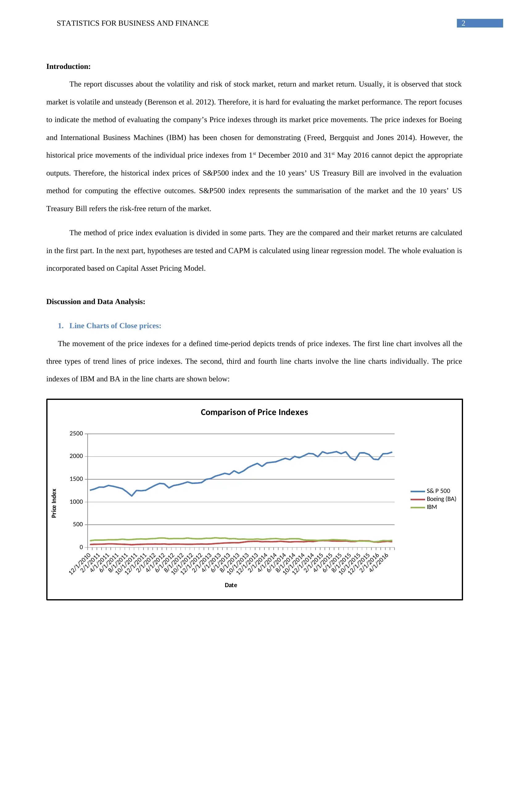
The movement of the price indexes for a defined time-period depicts trends of price indexes. The first line chart involves all the
three types of trend lines of price indexes. The second, third and fourth line charts involve the line charts individually. The price
indexes of IBM and BA in the line charts are shown below:
12/1/2010
2/1/2011
4/1/2011
6/1/2011
8/1/2011
10/1/2011
12/1/2011
2/1/2012
4/1/2012
6/1/2012
8/1/2012
10/1/2012
12/1/2012
2/1/2013
4/1/2013
6/1/2013
8/1/2013
10/1/2013
12/1/2013
2/1/2014
4/1/2014
6/1/2014
8/1/2014
10/1/2014
12/1/2014
2/1/2015
4/1/2015
6/1/2015
8/1/2015
10/1/2015
12/1/2015
2/1/2016
4/1/2016
0
500
1000
1500
2000
2500
Comparison of Price Indexes
S& P 500
Boeing (BA)
IBM
Date
Price Index
Introduction:
The report discusses about the volatility and risk of stock market, return and market return. Usually, it is observed that stock
market is volatile and unsteady (Berenson et al. 2012). Therefore, it is hard for evaluating the market performance. The report focuses
to indicate the method of evaluating the company’s Price indexes through its market price movements. The price indexes for Boeing
and International Business Machines (IBM) has been chosen for demonstrating (Freed, Bergquist and Jones 2014). However, the
historical price movements of the individual price indexes from 1st December 2010 and 31st May 2016 cannot depict the appropriate
outputs. Therefore, the historical index prices of S&P500 index and the 10 years’ US Treasury Bill are involved in the evaluation
method for computing the effective outcomes. S&P500 index represents the summarisation of the market and the 10 years’ US
Treasury Bill refers the risk-free return of the market.
The method of price index evaluation is divided in some parts. They are the compared and their market returns are calculated
in the first part. In the next part, hypotheses are tested and CAPM is calculated using linear regression model. The whole evaluation is
incorporated based on Capital Asset Pricing Model.
Discussion and Data Analysis:
1. Line Charts of Close prices:
The movement of the price indexes for a defined time-period depicts trends of price indexes. The first line chart involves all the
three types of trend lines of price indexes. The second, third and fourth line charts involve the line charts individually. The price
indexes of IBM and BA in the line charts are shown below:
12/1/2010
2/1/2011
4/1/2011
6/1/2011
8/1/2011
10/1/2011
12/1/2011
2/1/2012
4/1/2012
6/1/2012
8/1/2012
10/1/2012
12/1/2012
2/1/2013
4/1/2013
6/1/2013
8/1/2013
10/1/2013
12/1/2013
2/1/2014
4/1/2014
6/1/2014
8/1/2014
10/1/2014
12/1/2014
2/1/2015
4/1/2015
6/1/2015
8/1/2015
10/1/2015
12/1/2015
2/1/2016
4/1/2016
0
500
1000
1500
2000
2500
Comparison of Price Indexes
S& P 500
Boeing (BA)
IBM
Date
Price Index
⊘ This is a preview!⊘
Do you want full access?
Subscribe today to unlock all pages.
Trusted by 1+ million students worldwide
3STATISTICS FOR BUSINESS AND FINANCE
12/1/2010
2/1/2011
4/1/2011
6/1/2011
8/1/2011
10/1/2011
12/1/2011
2/1/2012
4/1/2012
6/1/2012
8/1/2012
10/1/2012
12/1/2012
2/1/2013
4/1/2013
6/1/2013
8/1/2013
10/1/2013
12/1/2013
2/1/2014
4/1/2014
6/1/2014
8/1/2014
10/1/2014
12/1/2014
2/1/2015
4/1/2015
6/1/2015
8/1/2015
10/1/2015
12/1/2015
2/1/2016
4/1/2016
0
500
1000
1500
2000
2500
S&P500 Price Index
S& P 500
Date
Price Index
12/1/2010
2/1/2011
4/1/2011
6/1/2011
8/1/2011
10/1/2011
12/1/2011
2/1/2012
4/1/2012
6/1/2012
8/1/2012
10/1/2012
12/1/2012
2/1/2013
4/1/2013
6/1/2013
8/1/2013
10/1/2013
12/1/2013
2/1/2014
4/1/2014
6/1/2014
8/1/2014
10/1/2014
12/1/2014
2/1/2015
4/1/2015
6/1/2015
8/1/2015
10/1/2015
12/1/2015
2/1/2016
4/1/2016
0
20
40
60
80
100
120
140
160
Boeing (BA) Price Index
Boeing (BA)
Date
Price Index
12/1/2010
2/1/2011
4/1/2011
6/1/2011
8/1/2011
10/1/2011
12/1/2011
2/1/2012
4/1/2012
6/1/2012
8/1/2012
10/1/2012
12/1/2012
2/1/2013
4/1/2013
6/1/2013
8/1/2013
10/1/2013
12/1/2013
2/1/2014
4/1/2014
6/1/2014
8/1/2014
10/1/2014
12/1/2014
2/1/2015
4/1/2015
6/1/2015
8/1/2015
10/1/2015
12/1/2015
2/1/2016
4/1/2016
0
50
100
150
200
250
IBM Price Index
IBM
Date
Price Index
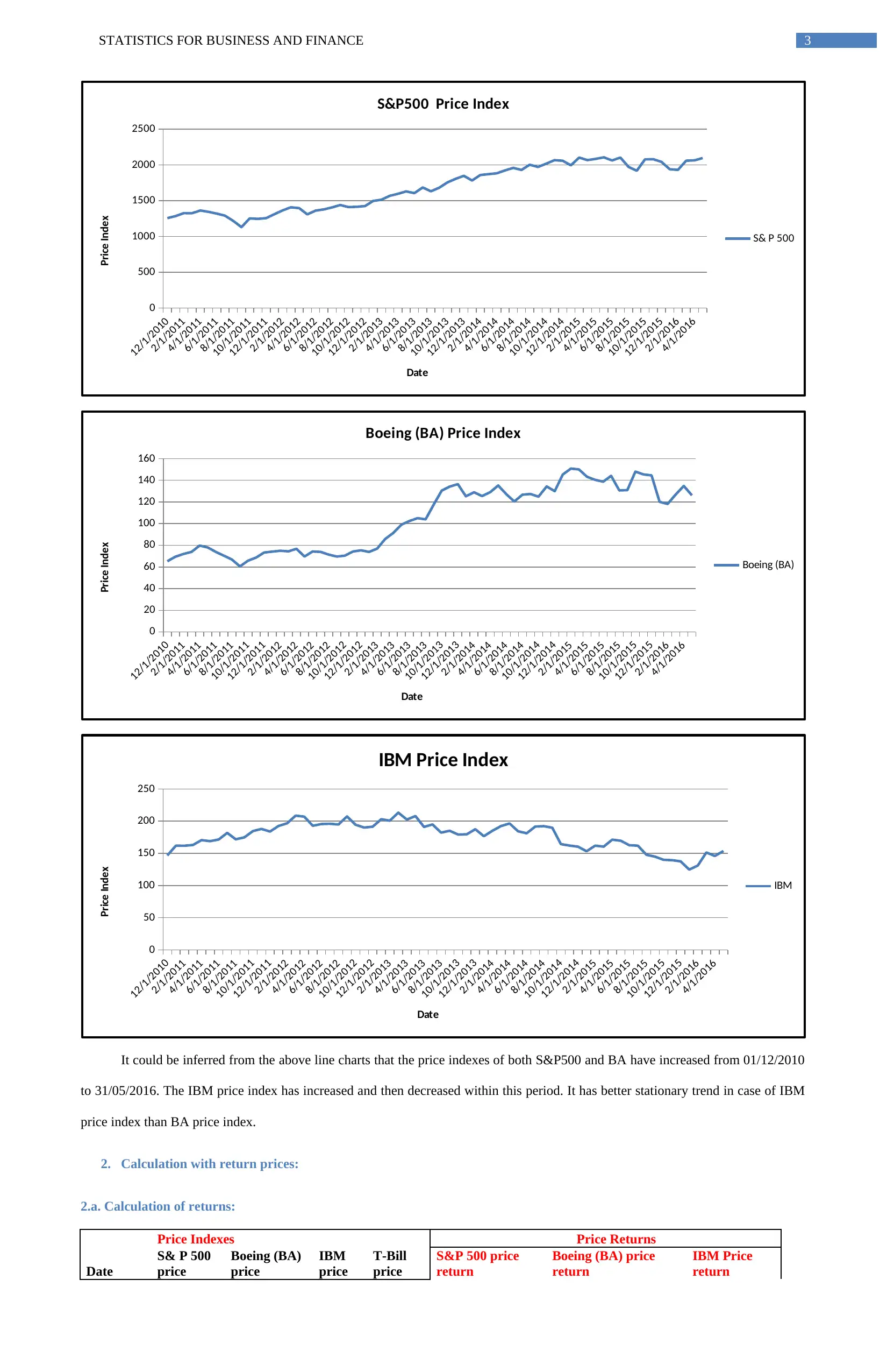
It could be inferred from the above line charts that the price indexes of both S&P500 and BA have increased from 01/12/2010
to 31/05/2016. The IBM price index has increased and then decreased within this period. It has better stationary trend in case of IBM
price index than BA price index.
2. Calculation with return prices:
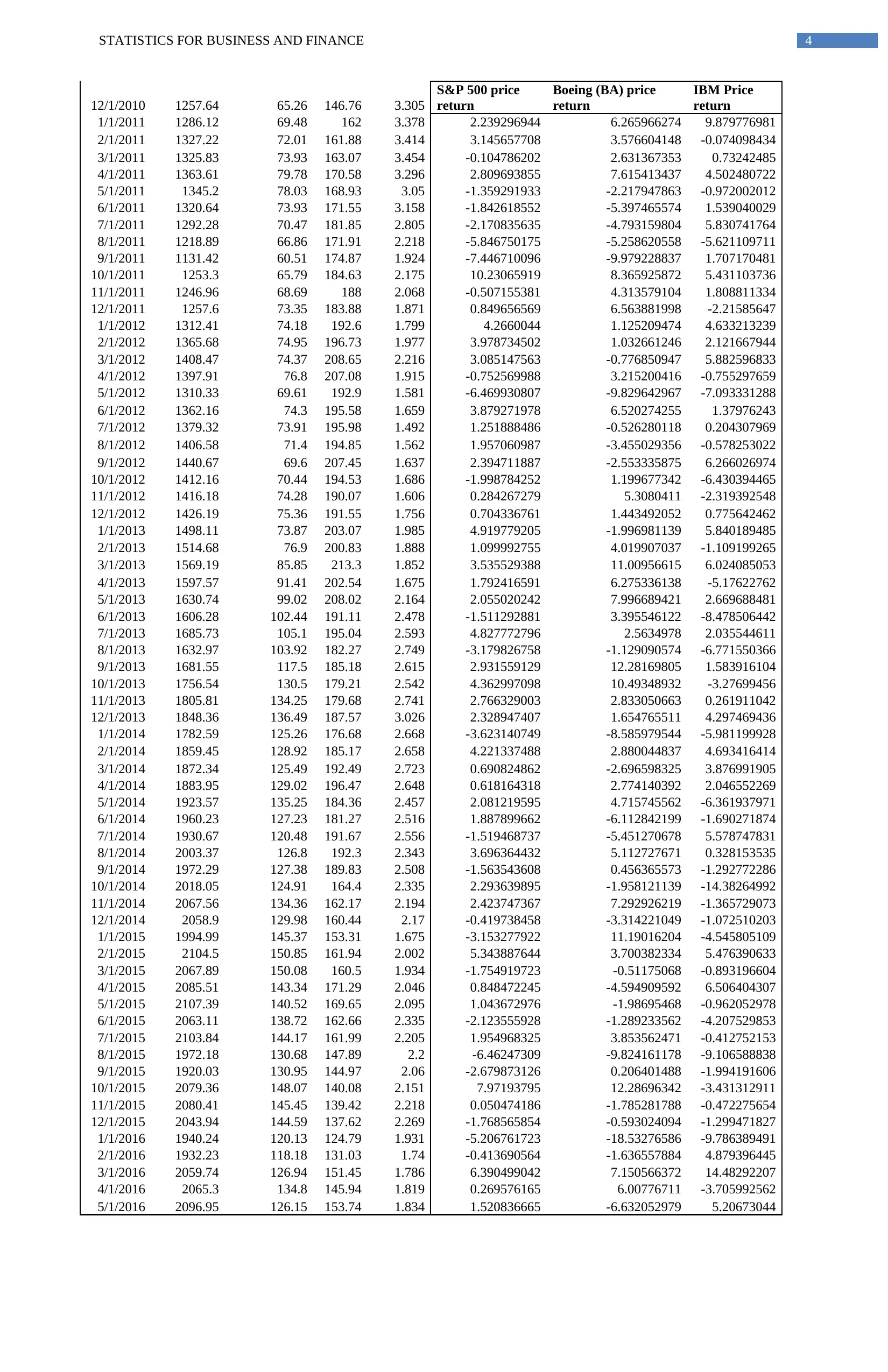
2.a. Calculation of returns:
Price Indexes Price Returns
Date
S& P 500
price
Boeing (BA)
price
IBM
price
T-Bill
price
S&P 500 price
return
Boeing (BA) price
return
IBM Price
return
12/1/2010
2/1/2011
4/1/2011
6/1/2011
8/1/2011
10/1/2011
12/1/2011
2/1/2012
4/1/2012
6/1/2012
8/1/2012
10/1/2012
12/1/2012
2/1/2013
4/1/2013
6/1/2013
8/1/2013
10/1/2013
12/1/2013
2/1/2014
4/1/2014
6/1/2014
8/1/2014
10/1/2014
12/1/2014
2/1/2015
4/1/2015
6/1/2015
8/1/2015
10/1/2015
12/1/2015
2/1/2016
4/1/2016
0
500
1000
1500
2000
2500
S&P500 Price Index
S& P 500
Date
Price Index
12/1/2010
2/1/2011
4/1/2011
6/1/2011
8/1/2011
10/1/2011
12/1/2011
2/1/2012
4/1/2012
6/1/2012
8/1/2012
10/1/2012
12/1/2012
2/1/2013
4/1/2013
6/1/2013
8/1/2013
10/1/2013
12/1/2013
2/1/2014
4/1/2014
6/1/2014
8/1/2014
10/1/2014
12/1/2014
2/1/2015
4/1/2015
6/1/2015
8/1/2015
10/1/2015
12/1/2015
2/1/2016
4/1/2016
0
20
40
60
80
100
120
140
160
Boeing (BA) Price Index
Boeing (BA)
Date
Price Index
12/1/2010
2/1/2011
4/1/2011
6/1/2011
8/1/2011
10/1/2011
12/1/2011
2/1/2012
4/1/2012
6/1/2012
8/1/2012
10/1/2012
12/1/2012
2/1/2013
4/1/2013
6/1/2013
8/1/2013
10/1/2013
12/1/2013
2/1/2014
4/1/2014
6/1/2014
8/1/2014
10/1/2014
12/1/2014
2/1/2015
4/1/2015
6/1/2015
8/1/2015
10/1/2015
12/1/2015
2/1/2016
4/1/2016
0
50
100
150
200
250
IBM Price Index
IBM
Date
Price Index
It could be inferred from the above line charts that the price indexes of both S&P500 and BA have increased from 01/12/2010
to 31/05/2016. The IBM price index has increased and then decreased within this period. It has better stationary trend in case of IBM
price index than BA price index.
2. Calculation with return prices:
2.a. Calculation of returns:
Price Indexes Price Returns
Date
S& P 500
price
Boeing (BA)
price
IBM
price
T-Bill
price
S&P 500 price
return
Boeing (BA) price
return
IBM Price
return
Paraphrase This Document
Need a fresh take? Get an instant paraphrase of this document with our AI Paraphraser
4STATISTICS FOR BUSINESS AND FINANCE
12/1/2010 1257.64 65.26 146.76 3.305
S&P 500 price
return
Boeing (BA) price
return
IBM Price
return
1/1/2011 1286.12 69.48 162 3.378 2.239296944 6.265966274 9.879776981
2/1/2011 1327.22 72.01 161.88 3.414 3.145657708 3.576604148 -0.074098434
3/1/2011 1325.83 73.93 163.07 3.454 -0.104786202 2.631367353 0.73242485
4/1/2011 1363.61 79.78 170.58 3.296 2.809693855 7.615413437 4.502480722
5/1/2011 1345.2 78.03 168.93 3.05 -1.359291933 -2.217947863 -0.972002012
6/1/2011 1320.64 73.93 171.55 3.158 -1.842618552 -5.397465574 1.539040029
7/1/2011 1292.28 70.47 181.85 2.805 -2.170835635 -4.793159804 5.830741764
8/1/2011 1218.89 66.86 171.91 2.218 -5.846750175 -5.258620558 -5.621109711
9/1/2011 1131.42 60.51 174.87 1.924 -7.446710096 -9.979228837 1.707170481
10/1/2011 1253.3 65.79 184.63 2.175 10.23065919 8.365925872 5.431103736
11/1/2011 1246.96 68.69 188 2.068 -0.507155381 4.313579104 1.808811334
12/1/2011 1257.6 73.35 183.88 1.871 0.849656569 6.563881998 -2.21585647
1/1/2012 1312.41 74.18 192.6 1.799 4.2660044 1.125209474 4.633213239
2/1/2012 1365.68 74.95 196.73 1.977 3.978734502 1.032661246 2.121667944
3/1/2012 1408.47 74.37 208.65 2.216 3.085147563 -0.776850947 5.882596833
4/1/2012 1397.91 76.8 207.08 1.915 -0.752569988 3.215200416 -0.755297659
5/1/2012 1310.33 69.61 192.9 1.581 -6.469930807 -9.829642967 -7.093331288
6/1/2012 1362.16 74.3 195.58 1.659 3.879271978 6.520274255 1.37976243
7/1/2012 1379.32 73.91 195.98 1.492 1.251888486 -0.526280118 0.204307969
8/1/2012 1406.58 71.4 194.85 1.562 1.957060987 -3.455029356 -0.578253022
9/1/2012 1440.67 69.6 207.45 1.637 2.394711887 -2.553335875 6.266026974
10/1/2012 1412.16 70.44 194.53 1.686 -1.998784252 1.199677342 -6.430394465
11/1/2012 1416.18 74.28 190.07 1.606 0.284267279 5.3080411 -2.319392548
12/1/2012 1426.19 75.36 191.55 1.756 0.704336761 1.443492052 0.775642462
1/1/2013 1498.11 73.87 203.07 1.985 4.919779205 -1.996981139 5.840189485
2/1/2013 1514.68 76.9 200.83 1.888 1.099992755 4.019907037 -1.109199265
3/1/2013 1569.19 85.85 213.3 1.852 3.535529388 11.00956615 6.024085053
4/1/2013 1597.57 91.41 202.54 1.675 1.792416591 6.275336138 -5.17622762
5/1/2013 1630.74 99.02 208.02 2.164 2.055020242 7.996689421 2.669688481
6/1/2013 1606.28 102.44 191.11 2.478 -1.511292881 3.395546122 -8.478506442
7/1/2013 1685.73 105.1 195.04 2.593 4.827772796 2.5634978 2.035544611
8/1/2013 1632.97 103.92 182.27 2.749 -3.179826758 -1.129090574 -6.771550366
9/1/2013 1681.55 117.5 185.18 2.615 2.931559129 12.28169805 1.583916104
10/1/2013 1756.54 130.5 179.21 2.542 4.362997098 10.49348932 -3.27699456
11/1/2013 1805.81 134.25 179.68 2.741 2.766329003 2.833050663 0.261911042
12/1/2013 1848.36 136.49 187.57 3.026 2.328947407 1.654765511 4.297469436
1/1/2014 1782.59 125.26 176.68 2.668 -3.623140749 -8.585979544 -5.981199928
2/1/2014 1859.45 128.92 185.17 2.658 4.221337488 2.880044837 4.693416414
3/1/2014 1872.34 125.49 192.49 2.723 0.690824862 -2.696598325 3.876991905
4/1/2014 1883.95 129.02 196.47 2.648 0.618164318 2.774140392 2.046552269
5/1/2014 1923.57 135.25 184.36 2.457 2.081219595 4.715745562 -6.361937971
6/1/2014 1960.23 127.23 181.27 2.516 1.887899662 -6.112842199 -1.690271874
7/1/2014 1930.67 120.48 191.67 2.556 -1.519468737 -5.451270678 5.578747831
8/1/2014 2003.37 126.8 192.3 2.343 3.696364432 5.112727671 0.328153535
9/1/2014 1972.29 127.38 189.83 2.508 -1.563543608 0.456365573 -1.292772286
10/1/2014 2018.05 124.91 164.4 2.335 2.293639895 -1.958121139 -14.38264992
11/1/2014 2067.56 134.36 162.17 2.194 2.423747367 7.292926219 -1.365729073
12/1/2014 2058.9 129.98 160.44 2.17 -0.419738458 -3.314221049 -1.072510203
1/1/2015 1994.99 145.37 153.31 1.675 -3.153277922 11.19016204 -4.545805109
2/1/2015 2104.5 150.85 161.94 2.002 5.343887644 3.700382334 5.476390633
3/1/2015 2067.89 150.08 160.5 1.934 -1.754919723 -0.51175068 -0.893196604
4/1/2015 2085.51 143.34 171.29 2.046 0.848472245 -4.594909592 6.506404307
5/1/2015 2107.39 140.52 169.65 2.095 1.043672976 -1.98695468 -0.962052978
6/1/2015 2063.11 138.72 162.66 2.335 -2.123555928 -1.289233562 -4.207529853
7/1/2015 2103.84 144.17 161.99 2.205 1.954968325 3.853562471 -0.412752153
8/1/2015 1972.18 130.68 147.89 2.2 -6.46247309 -9.824161178 -9.106588838
9/1/2015 1920.03 130.95 144.97 2.06 -2.679873126 0.206401488 -1.994191606
10/1/2015 2079.36 148.07 140.08 2.151 7.97193795 12.28696342 -3.431312911
11/1/2015 2080.41 145.45 139.42 2.218 0.050474186 -1.785281788 -0.472275654
12/1/2015 2043.94 144.59 137.62 2.269 -1.768565854 -0.593024094 -1.299471827
1/1/2016 1940.24 120.13 124.79 1.931 -5.206761723 -18.53276586 -9.786389491
2/1/2016 1932.23 118.18 131.03 1.74 -0.413690564 -1.636557884 4.879396445
3/1/2016 2059.74 126.94 151.45 1.786 6.390499042 7.150566372 14.48292207
4/1/2016 2065.3 134.8 145.94 1.819 0.269576165 6.00776711 -3.705992562
5/1/2016 2096.95 126.15 153.74 1.834 1.520836665 -6.632052979 5.20673044
5STATISTICS FOR BUSINESS AND FINANCE
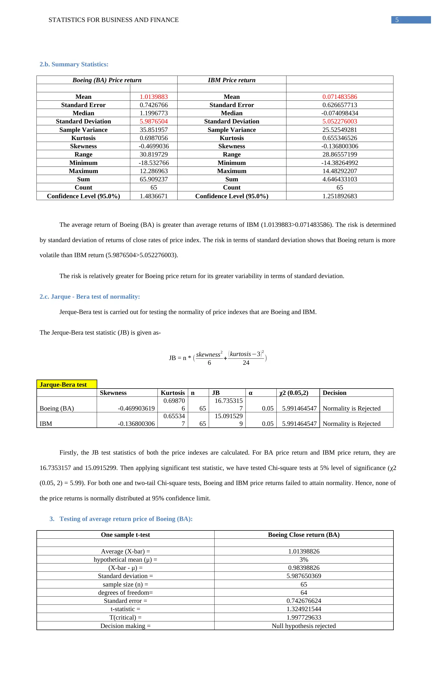
2.b. Summary Statistics:
Boeing (BA) Price return IBM Price return
Mean 1.0139883 Mean 0.071483586
Standard Error 0.7426766 Standard Error 0.626657713
Median 1.1996773 Median -0.074098434
Standard Deviation 5.9876504 Standard Deviation 5.052276003
Sample Variance 35.851957 Sample Variance 25.52549281
Kurtosis 0.6987056 Kurtosis 0.655346526
Skewness -0.4699036 Skewness -0.136800306
Range 30.819729 Range 28.86557199
Minimum -18.532766 Minimum -14.38264992
Maximum 12.286963 Maximum 14.48292207
Sum 65.909237 Sum 4.646433103
Count 65 Count 65
Confidence Level (95.0%) 1.4836671 Confidence Level (95.0%) 1.251892683
The average return of Boeing (BA) is greater than average returns of IBM (1.0139883>0.071483586). The risk is determined
by standard deviation of returns of close rates of price index. The risk in terms of standard deviation shows that Boeing return is more
volatile than IBM return (5.9876504>5.052276003).
The risk is relatively greater for Boeing price return for its greater variability in terms of standard deviation.
2.c. Jarque - Bera test of normality:
Jerque-Bera test is carried out for testing the normality of price indexes that are Boeing and IBM.
The Jerque-Bera test statistic (JB) is given as-
JB = n * ( skewness2
6 + ( kurtosis−3 ) 2
24 )
Jarque-Bera test
Skewness Kurtosis n JB α χ2 (0.05,2) Decision
Boeing (BA) -0.469903619
0.69870
6 65
16.735315
7 0.05 5.991464547 Normality is Rejected
IBM -0.136800306
0.65534
7 65
15.091529
9 0.05 5.991464547 Normality is Rejected
Firstly, the JB test statistics of both the price indexes are calculated. For BA price return and IBM price return, they are
16.7353157 and 15.0915299. Then applying significant test statistic, we have tested Chi-square tests at 5% level of significance (χ2
(0.05, 2) = 5.99). For both one and two-tail Chi-square tests, Boeing and IBM price returns failed to attain normality. Hence, none of
the price returns is normally distributed at 95% confidence limit.
3. Testing of average return price of Boeing (BA):
One sample t-test Boeing Close return (BA)
Average (X-bar) = 1.01398826
hypothetical mean (μ) = 3%
(X-bar - μ) = 0.98398826
Standard deviation = 5.987650369
sample size (n) = 65
degrees of freedom= 64
Standard error = 0.742676624
t-statistic = 1.324921544
T(critical) = 1.997729633
Decision making = Null hypothesis rejected
⊘ This is a preview!⊘
Do you want full access?
Subscribe today to unlock all pages.
Trusted by 1+ million students worldwide
6STATISTICS FOR BUSINESS AND FINANCE
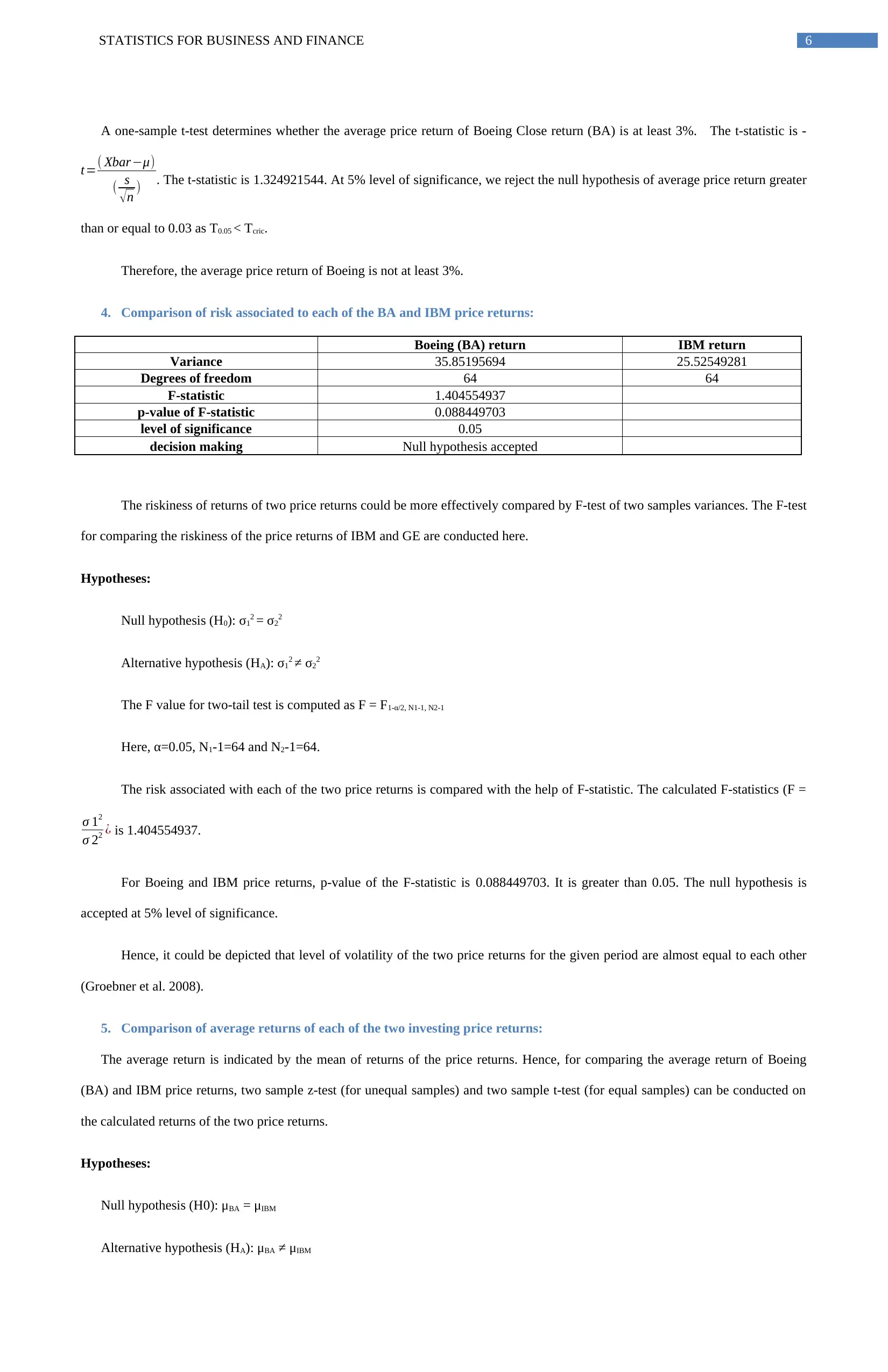
A one-sample t-test determines whether the average price return of Boeing Close return (BA) is at least 3%. The t-statistic is -
t=( Xbar−μ)
( s
√n ) . The t-statistic is 1.324921544. At 5% level of significance, we reject the null hypothesis of average price return greater
than or equal to 0.03 as T0.05 < Tcric.
Therefore, the average price return of Boeing is not at least 3%.
4. Comparison of risk associated to each of the BA and IBM price returns:
Boeing (BA) return IBM return
Variance 35.85195694 25.52549281
Degrees of freedom 64 64
F-statistic 1.404554937
p-value of F-statistic 0.088449703
level of significance 0.05
decision making Null hypothesis accepted
The riskiness of returns of two price returns could be more effectively compared by F-test of two samples variances. The F-test
for comparing the riskiness of the price returns of IBM and GE are conducted here.
Hypotheses:
Null hypothesis (H0): σ12 = σ22
Alternative hypothesis (HA): σ12 ≠ σ22
The F value for two-tail test is computed as F = F1-α/2, N1-1, N2-1
Here, α=0.05, N1-1=64 and N2-1=64.
The risk associated with each of the two price returns is compared with the help of F-statistic. The calculated F-statistics (F =
σ 12
σ 22 ¿ is 1.404554937.
For Boeing and IBM price returns, p-value of the F-statistic is 0.088449703. It is greater than 0.05. The null hypothesis is
accepted at 5% level of significance.
Hence, it could be depicted that level of volatility of the two price returns for the given period are almost equal to each other
(Groebner et al. 2008).
5. Comparison of average returns of each of the two investing price returns:
The average return is indicated by the mean of returns of the price returns. Hence, for comparing the average return of Boeing
(BA) and IBM price returns, two sample z-test (for unequal samples) and two sample t-test (for equal samples) can be conducted on
the calculated returns of the two price returns.
Hypotheses:
Null hypothesis (H0): μBA = μIBM
Alternative hypothesis (HA): μBA ≠ μIBM
Paraphrase This Document
Need a fresh take? Get an instant paraphrase of this document with our AI Paraphraser

7STATISTICS FOR BUSINESS AND FINANCE
The z-statistic is given as z¿ ( Xbar −μ)
( σ
√n ) and t-statistic is given as t=( Xbar−μ)
( s
√ n ) .
Z-test of equality of means of two samples:
z-Test: Two Sample for Means
Boeing (BA) returns IBM returns
Mean 1.01398826 0.071483586
Known Variance 35.8519 25.5254
Observations 65 65
Hypothesized Mean Difference 0
z 0.969920863
P(Z<=z) one-tail 0.16604297
z Critical one-tail 1.644853627
P(Z<=z) two-tail 0.33208594
z Critical two-tail 1.959963985
decision making Null hypothesis accepted
For comparing the average returns of each of the two investing price returns, a z-test is applied. The variances are known for
each of the price returns. The calculated z-statistic is 0.9699. The p-value for two-tail z-statistic is 0.332 (>0.05). Therefore, we can
reject the null hypothesis of equality of averages of returns of two price returns at 5% level of significance.
Two-sample t-test of equality of means for unequal variances:
t-Test: Two-Sample Assuming Unequal Variances
Boeing (BA) return IBM return
Mean 1.01398826 0.07148359
Variance 35.85195694 25.5254928
Observations 65 65
Hypothesized Mean Difference 0
df 124
t Stat 0.96991968
P(T<=t) one-tail 0.166987311
t Critical one-tail 1.657234971
P(T<=t) two-tail 0.333974621
t Critical two-tail 1.979280091
decision making Null hypothesis accepted
The t-test assuming equal variances of BA and IBM price returns gives the t-statistic 0.96991968. The p-value of the two-tail t-
test is found to be 0.333974621. The level of significance is 5%, which is lesser than calculated p-value. Therefore, we cannot reject
the null hypothesis of equality of averages of both the price returns.
Inference:
According to the price return averages and price return standard deviations (risk), an equality is established. Hence, we cannot
draw firm decision to choose any one price returns between BA and IBM. Hence, we further proceed with both of them. Next, we are
willing to excess price return, excess market return and CAPM of both the price returns. With the help of these, we can find the
volatility of both the price returns. The preferable price return would be distinguished after that.
6. Calculation of Excess Return and Excess Return:
Excess Return Excess Return Excess Market Return
Boeing Excess return (BA) IBM Excess return
BA IBM
ytBA ytIBM xt
2.887966274 6.501776981 -1.138703056
0.162604148 -3.488098434 -0.268342292
-0.822632647 -2.72157515 -3.558786202
4.319413437 1.206480722 -0.486306145
-5.267947863 -4.022002012 -4.409291933
-8.555465574 -1.618959971 -5.000618552
-7.598159804 3.025741764 -4.975835635
8STATISTICS FOR BUSINESS AND FINANCE
-7.476620558 -7.839109711 -8.064750175
-11.90322884 -0.216829519 -9.370710096
6.190925872 3.256103736 8.055659186
2.245579104 -0.259188666 -2.575155381
4.692881998 -4.08685647 -1.021343431
-0.673790526 2.834213239 2.4670044
-0.944338754 0.144667944 2.001734502
-2.992850947 3.666596833 0.869147563
1.300200416 -2.670297659 -2.667569988
-11.41064297 -8.674331288 -8.050930807
4.861274255 -0.27923757 2.220271978
-2.018280118 -1.287692031 -0.240111514
-5.017029356 -2.140253022 0.395060987
-4.190335875 4.629026974 0.757711887
-0.486322658 -8.116394465 -3.684784252
3.7020411 -3.925392548 -1.321732721
-0.312507948 -0.980357538 -1.051663239
-3.981981139 3.855189485 2.934779205
2.131907037 -2.997199265 -0.788007245
9.157566153 4.172085053 1.683529388
4.600336138 -6.85122762 0.117416591
5.832689421 0.505688481 -0.108979758
0.917546122 -10.95650644 -3.989292881
-0.0295022 -0.557455389 2.234772796
-3.878090574 -9.520550366 -5.928826758
9.666698047 -1.031083896 0.316559129
7.951489318 -5.81899456 1.820997098
0.092050663 -2.479088958 0.025329003
-1.371234489 1.271469436 -0.697052593
-11.25397954 -8.649199928 -6.291140749
0.222044837 2.035416414 1.563337488
-5.419598325 1.153991905 -2.032175138
0.126140392 -0.601447731 -2.029835682
2.258745562 -8.818937971 -0.375780405
-8.628842199 -4.206271874 -0.628100338
-8.007270678 3.022747831 -4.075468737
2.769727671 -2.014846465 1.353364432
-2.051634427 -3.800772286 -4.071543608
-4.293121139 -16.71764992 -0.041360105
5.098926219 -3.559729073 0.229747367
-5.484221049 -3.242510203 -2.589738458
9.515162035 -6.220805109 -4.828277922
1.698382334 3.474390633 3.341887644
-2.44575068 -2.827196604 -3.688919723
-6.640909592 4.460404307 -1.197527755
-4.08195468 -3.057052978 -1.051327024
-3.624233562 -6.542529853 -4.458555928
1.648562471 -2.617752153 -0.250031675
-12.02416118 -11.30658884 -8.66247309
-1.853598512 -4.054191606 -4.739873126
10.13596342 -5.582312911 5.82093795
-4.003281788 -2.690275654 -2.167525814
-2.862024094 -3.568471827 -4.037565854
-20.46376586 -11.71738949 -7.137761723
-3.376557884 3.139396445 -2.153690564
5.364566372 12.69692207 4.604499042
4.18876711 -5.524992562 -1.549423835
-8.466052979 3.37273044 -0.313163335
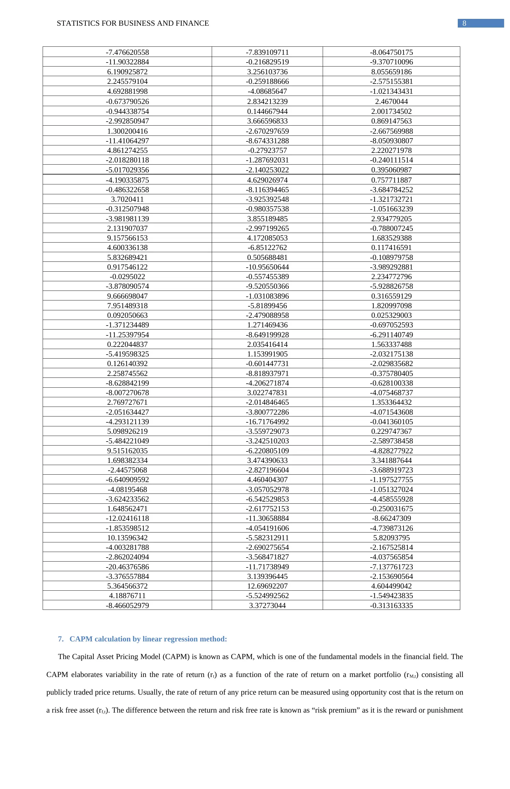
7. CAPM calculation by linear regression method:
The Capital Asset Pricing Model (CAPM) is known as CAPM, which is one of the fundamental models in the financial field. The
CAPM elaborates variability in the rate of return (rt) as a function of the rate of return on a market portfolio (rM,t) consisting all
publicly traded price returns. Usually, the rate of return of any price return can be measured using opportunity cost that is the return on
a risk free asset (rf,t). The difference between the return and risk free rate is known as “risk premium” as it is the reward or punishment
-7.476620558 -7.839109711 -8.064750175
-11.90322884 -0.216829519 -9.370710096
6.190925872 3.256103736 8.055659186
2.245579104 -0.259188666 -2.575155381
4.692881998 -4.08685647 -1.021343431
-0.673790526 2.834213239 2.4670044
-0.944338754 0.144667944 2.001734502
-2.992850947 3.666596833 0.869147563
1.300200416 -2.670297659 -2.667569988
-11.41064297 -8.674331288 -8.050930807
4.861274255 -0.27923757 2.220271978
-2.018280118 -1.287692031 -0.240111514
-5.017029356 -2.140253022 0.395060987
-4.190335875 4.629026974 0.757711887
-0.486322658 -8.116394465 -3.684784252
3.7020411 -3.925392548 -1.321732721
-0.312507948 -0.980357538 -1.051663239
-3.981981139 3.855189485 2.934779205
2.131907037 -2.997199265 -0.788007245
9.157566153 4.172085053 1.683529388
4.600336138 -6.85122762 0.117416591
5.832689421 0.505688481 -0.108979758
0.917546122 -10.95650644 -3.989292881
-0.0295022 -0.557455389 2.234772796
-3.878090574 -9.520550366 -5.928826758
9.666698047 -1.031083896 0.316559129
7.951489318 -5.81899456 1.820997098
0.092050663 -2.479088958 0.025329003
-1.371234489 1.271469436 -0.697052593
-11.25397954 -8.649199928 -6.291140749
0.222044837 2.035416414 1.563337488
-5.419598325 1.153991905 -2.032175138
0.126140392 -0.601447731 -2.029835682
2.258745562 -8.818937971 -0.375780405
-8.628842199 -4.206271874 -0.628100338
-8.007270678 3.022747831 -4.075468737
2.769727671 -2.014846465 1.353364432
-2.051634427 -3.800772286 -4.071543608
-4.293121139 -16.71764992 -0.041360105
5.098926219 -3.559729073 0.229747367
-5.484221049 -3.242510203 -2.589738458
9.515162035 -6.220805109 -4.828277922
1.698382334 3.474390633 3.341887644
-2.44575068 -2.827196604 -3.688919723
-6.640909592 4.460404307 -1.197527755
-4.08195468 -3.057052978 -1.051327024
-3.624233562 -6.542529853 -4.458555928
1.648562471 -2.617752153 -0.250031675
-12.02416118 -11.30658884 -8.66247309
-1.853598512 -4.054191606 -4.739873126
10.13596342 -5.582312911 5.82093795
-4.003281788 -2.690275654 -2.167525814
-2.862024094 -3.568471827 -4.037565854
-20.46376586 -11.71738949 -7.137761723
-3.376557884 3.139396445 -2.153690564
5.364566372 12.69692207 4.604499042
4.18876711 -5.524992562 -1.549423835
-8.466052979 3.37273044 -0.313163335
7. CAPM calculation by linear regression method:
The Capital Asset Pricing Model (CAPM) is known as CAPM, which is one of the fundamental models in the financial field. The
CAPM elaborates variability in the rate of return (rt) as a function of the rate of return on a market portfolio (rM,t) consisting all
publicly traded price returns. Usually, the rate of return of any price return can be measured using opportunity cost that is the return on
a risk free asset (rf,t). The difference between the return and risk free rate is known as “risk premium” as it is the reward or punishment
⊘ This is a preview!⊘
Do you want full access?
Subscribe today to unlock all pages.
Trusted by 1+ million students worldwide
9STATISTICS FOR BUSINESS AND FINANCE
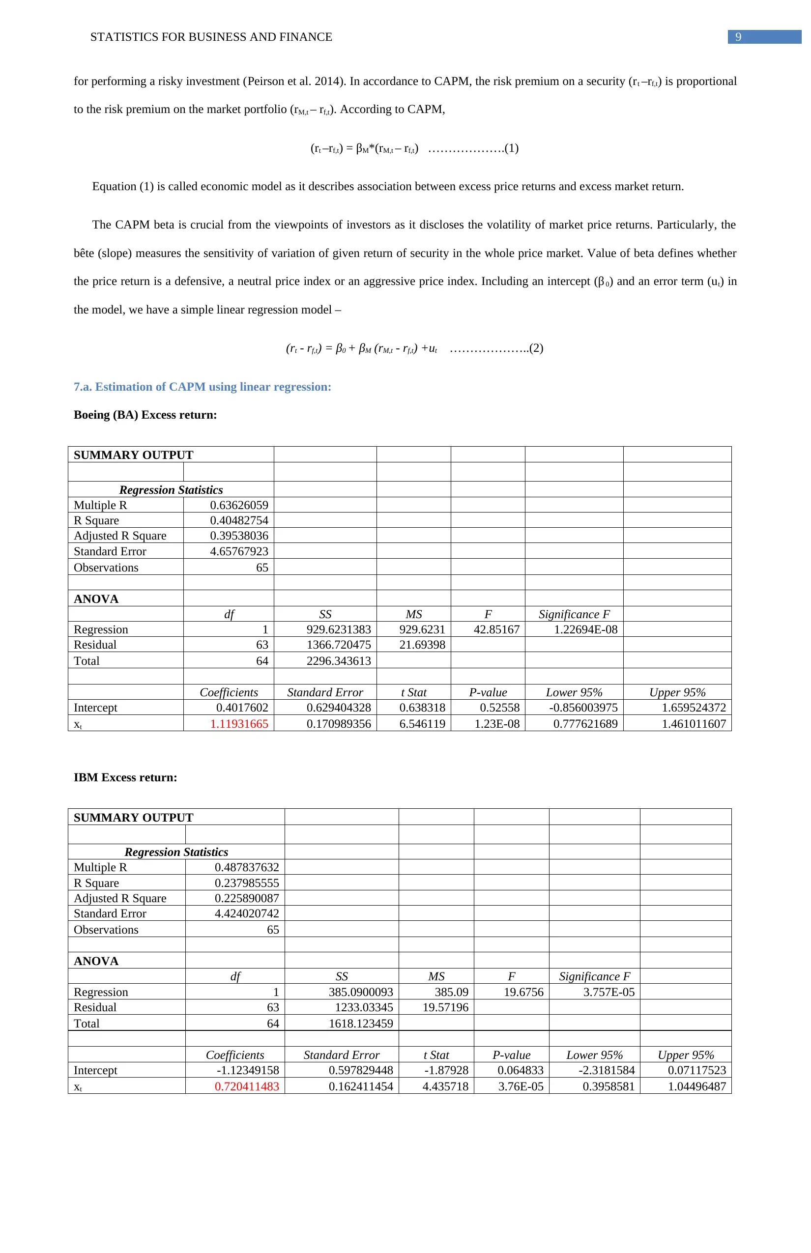
for performing a risky investment (Peirson et al. 2014). In accordance to CAPM, the risk premium on a security (rt –rf,t) is proportional
to the risk premium on the market portfolio (rM,t – rf,t). According to CAPM,
(rt –rf,t) = βM*(rM,t – rf,t) ……………….(1)
Equation (1) is called economic model as it describes association between excess price returns and excess market return.
The CAPM beta is crucial from the viewpoints of investors as it discloses the volatility of market price returns. Particularly, the
bête (slope) measures the sensitivity of variation of given return of security in the whole price market. Value of beta defines whether
the price return is a defensive, a neutral price index or an aggressive price index. Including an intercept (β 0) and an error term (ut) in
the model, we have a simple linear regression model –
(rt - rf,t) = β0 + βM (rM,t - rf,t) +ut ………………..(2)
7.a. Estimation of CAPM using linear regression:
Boeing (BA) Excess return:
SUMMARY OUTPUT
Regression Statistics
Multiple R 0.63626059
R Square 0.40482754
Adjusted R Square 0.39538036
Standard Error 4.65767923
Observations 65
ANOVA
df SS MS F Significance F
Regression 1 929.6231383 929.6231 42.85167 1.22694E-08
Residual 63 1366.720475 21.69398
Total 64 2296.343613
Coefficients Standard Error t Stat P-value Lower 95% Upper 95%
Intercept 0.4017602 0.629404328 0.638318 0.52558 -0.856003975 1.659524372
xt 1.11931665 0.170989356 6.546119 1.23E-08 0.777621689 1.461011607
IBM Excess return:
SUMMARY OUTPUT
Regression Statistics
Multiple R 0.487837632
R Square 0.237985555
Adjusted R Square 0.225890087
Standard Error 4.424020742
Observations 65
ANOVA
df SS MS F Significance F
Regression 1 385.0900093 385.09 19.6756 3.757E-05
Residual 63 1233.03345 19.57196
Total 64 1618.123459
Coefficients Standard Error t Stat P-value Lower 95% Upper 95%
Intercept -1.12349158 0.597829448 -1.87928 0.064833 -2.3181584 0.07117523
xt 0.720411483 0.162411454 4.435718 3.76E-05 0.3958581 1.04496487
Paraphrase This Document
Need a fresh take? Get an instant paraphrase of this document with our AI Paraphraser
10STATISTICS FOR BUSINESS AND FINANCE
7.b. Interpretation of Coefficients:
The calculated β-value for Boeing excess return and Excess market return is 1.11931665. The calculated β-value for IBM excess
return and Excess market return is 0.720411483. The calculated β-values define that BA price indexes are 111.93% less volatile than
the market, whereas the volatility level of IBM compared to the market is 72.04%. Therefore, it can be stated that Boeing (BA) is
highly volatile than IBM. Therefore, Boeing (BA) is considered to be more profitable than IBM price returns.
7.c. Interpretation of R2:
The linear regression tables describe that the values of R2 of BA and IBM are 0.40482754 and 0.237985555. The R2 indicates
the relationship of the dependent variable with the independent variable. Hence, from the values of multiple R2 of the two price returns
it could be stated that Boeing (BA) excess return (40.48%) is more associated than the association of IBM (23.80%).
7.d. Construction of 95% confidence interval for Slope Efficient:
Confidence Interval of IBM Price Return:
A. For Boeing (BA) price return, slope (β1) = 1.11931665, Standard Error = 0.170989356, d.f. = 64, t-value = 6.546119. Hence,
the 95% confidence interval for the slope coefficient would be (0.777621689, 1.461011607).
B. For IBM price return, slope (β1) = 0.720411483, Standard Error = 0.162411454, d.f. = 64, t-value = 4.435718. Hence, the 95%
confidence interval for the slope coefficient would be (0.3958581, 1.04496487).
8. Preferable neutral Price Return:
The testing of aggressiveness of the excess price returns needs the following hypothesis:
Null hypothesis (H0): β1 = 1
Alternative hypothesis (H1): β1 < 1
For BA price returns, β1 is 1.11931665 along with the standard error (SE) 0.170989356. The “residual degrees of freedom” is
63 and calculated p-value is 0.0. Hence, t = β1/ SE = 6.546119.
For IBM price indexes, β1 is 0.720411483 along with the standard error (SE) 0.162411454. The “residual degrees of freedom”
is 63 and calculated p-value is 0.0. Hence, t = β1/ SE = 4.435718.
For both the excess price returns, the p-values are positive t-value and equal degrees of freedom 64. The 95% confidence intervals
for beta values of both BA and IBM price returns are (0.777621689, 1.461011607) and (0.3958581, 1.04496487). The confidence
intervals near to 0 refers more neutral nature for price excess return. The confidence intervals of t-statistics indicate that IBM price
return is more neutral (Moffett, Stonehill and Eiteman 2014).
9. Normal Probability Plot in OLS:
IBM Ecess Price return residual plot:
11STATISTICS FOR BUSINESS AND FINANCE
0.769230769230769
3.84615384615385
6.92307692307692
10
13.0769230769231
16.1538461538462
19.2307692307692
22.3076923076923
25.3846153846154
28.4615384615385
31.5384615384615
34.6153846153845
37.6923076923077
40.7692307692308
43.8461538461539
46.923076923077
50
53.0769230769231
56.153846153846
59.2307692307693
62.3076923076922
65.3846153846155
68.4615384615385
71.5384615384613
74.6153846153845
77.6923076923077
80.7692307692309
83.8461538461539
86.9230769230769
90
93.0769230769231
96.1538461538459
99.2307692307692
-20
-15
-10
-5
0
5
10
15
Normal Probability Plot
Sample Percentile
ytIBM
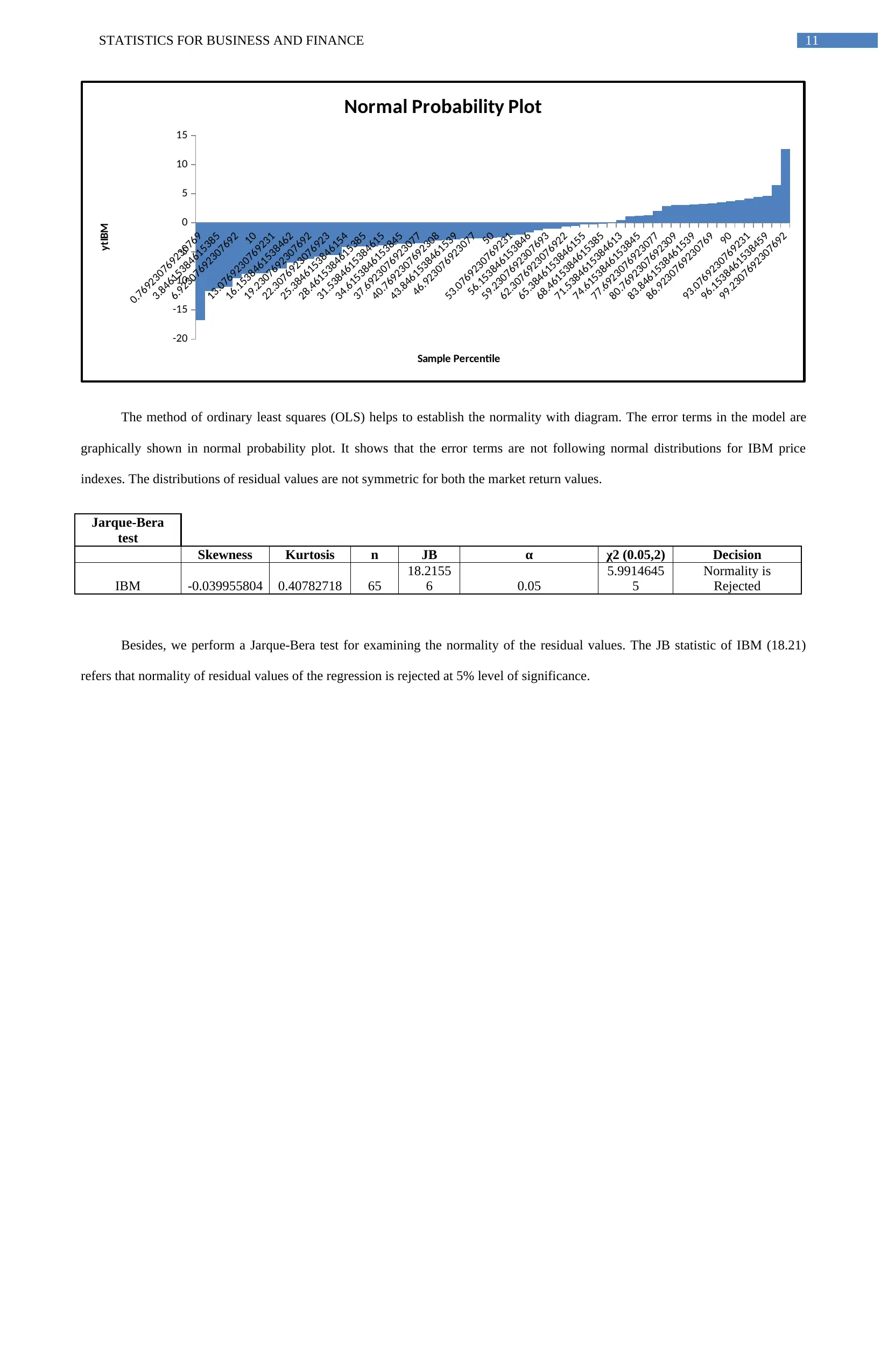
The method of ordinary least squares (OLS) helps to establish the normality with diagram. The error terms in the model are
graphically shown in normal probability plot. It shows that the error terms are not following normal distributions for IBM price
indexes. The distributions of residual values are not symmetric for both the market return values.
Jarque-Bera
test
Skewness Kurtosis n JB α χ2 (0.05,2) Decision
IBM -0.039955804 0.40782718 65
18.2155
6 0.05
5.9914645
5
Normality is
Rejected
Besides, we perform a Jarque-Bera test for examining the normality of the residual values. The JB statistic of IBM (18.21)
refers that normality of residual values of the regression is rejected at 5% level of significance.
0.769230769230769
3.84615384615385
6.92307692307692
10
13.0769230769231
16.1538461538462
19.2307692307692
22.3076923076923
25.3846153846154
28.4615384615385
31.5384615384615
34.6153846153845
37.6923076923077
40.7692307692308
43.8461538461539
46.923076923077
50
53.0769230769231
56.153846153846
59.2307692307693
62.3076923076922
65.3846153846155
68.4615384615385
71.5384615384613
74.6153846153845
77.6923076923077
80.7692307692309
83.8461538461539
86.9230769230769
90
93.0769230769231
96.1538461538459
99.2307692307692
-20
-15
-10
-5
0
5
10
15
Normal Probability Plot
Sample Percentile
ytIBM
The method of ordinary least squares (OLS) helps to establish the normality with diagram. The error terms in the model are
graphically shown in normal probability plot. It shows that the error terms are not following normal distributions for IBM price
indexes. The distributions of residual values are not symmetric for both the market return values.
Jarque-Bera
test
Skewness Kurtosis n JB α χ2 (0.05,2) Decision
IBM -0.039955804 0.40782718 65
18.2155
6 0.05
5.9914645
5
Normality is
Rejected
Besides, we perform a Jarque-Bera test for examining the normality of the residual values. The JB statistic of IBM (18.21)
refers that normality of residual values of the regression is rejected at 5% level of significance.
⊘ This is a preview!⊘
Do you want full access?
Subscribe today to unlock all pages.
Trusted by 1+ million students worldwide
1 out of 13
Related Documents


Your All-in-One AI-Powered Toolkit for Academic Success.
+13062052269
info@desklib.com
Available 24*7 on WhatsApp / Email
![[object Object]](/_next/static/media/star-bottom.7253800d.svg)
Unlock your academic potential
Copyright © 2020–2026 A2Z Services. All Rights Reserved. Developed and managed by ZUCOL.